4 Statistical inference for two-way tables
4.1 Introduction
In this section we continue the discussion of methods of analysis for two-way contingency tables that was begun in Section 2.4.1. We will use again the example from the European Social Survey that was introduced early in Section 2.2. The two variables in the example are a person’s sex and his or her attitude toward income redistribution measured as an ordinal variable with five levels. The two-way table of these variables in the sample is shown again for convenience in Table 4.1, including both the frequencies and the conditional proportions for attitude given sex.
|
Sex |
Agree strongly | Agree | Neither agree nor disagree | Disagree | Disagree strongly | Total |
|---|---|---|---|---|---|---|
| Male | 160 | 439 | 187 | 200 | 41 | 1027 |
| (0.156) | (0.428) | (0.182) | (0.195) | (0.040) | (1.0) | |
| Female | 206 | 651 | 239 | 187 | 34 | 1317 |
| (0.156) | (0.494) | (0.182) | (0.142) | (0.026) | (1.0) | |
| Total | 366 | 1090 | 426 | 387 | 75 | 2344 |
| (0.156) | (0.465) | (0.182) | (0.165) | (0.032) | (1.0) |
Unlike in Section 2.4.1, we will now go beyond description of sample distributions and into statistical inference. The observed data are thus treated as a sample from a population, and we wish to draw conclusions about the population distributions of the variables. In particular, we want to examine whether the sample provides evidence that the two variables in the table are associated in the population — in the example, whether attitude depends on sex in the population. This is done using a statistical significance test known as \(\chi^{2}\) test of independence. We will use it also as a vehicle for introducing the basic ideas of significance testing in general.
This initial explanation of significance tests is be lengthy and detailed, because it is important to gain a good understanding of these fundamental concepts from the beginning. From then on, the same ideas will be used repeatedly throughout the rest of the course, and in practically all statistical methods that you may encounter in the future. You will then be able to draw on what you will have learned in this chapter, and that learning will also be reinforced through repeated appearances of the same concepts in different contexts. It will then not be necessary to restate the basic ideas of the tools of inference in similar detail. A short summary of the \(\chi^{2}\) test considered in this chapter is given again at the end of the chapter, in Section 4.4.
4.2 Significance tests
A significance test is a method of statistical inference that is used to assess the plausibility of hypotheses about a population. A hypothesis is a question about population distributions, formulated as a claim about those distributions. For the test considered in this chapter, the question is whether or not the two variables in a contingency table are associated in the population. In the example we want to know whether men and women have the same distribution of attitudes towards income redistribution in the population. For significance testing, this question is expressed as the claim “The distribution of attitudes towards income redistribution is the same for men and women”, to which we want to identify the correct response, either “Yes, it is” or “No, it isn’t”.
In trying to answer such questions, we are faced with the complication that we only have information from a sample. For example, in Table 4.1 the conditional distributions of attitude are certainly not identical for men and women. According to the definition in Section 2.4.3, this shows that sex and attitude are associated in the sample. This, however, does not prove that they are also associated in the population. Because of sampling variation, the two conditional distributions are very unlike to be exactly identical in a sample even if they are the same in the population. In other words, the hypothesis will not be exactly true in a sample even if it is true in the population.
On the other hand, some sample values differ from the values claimed by the hypothesis by so much that it would be difficult to explain them as a result of sampling variation alone. For example, if we had observed a sample where 99% of the men but only 1% of the women disagreed with the attitude statement, it would seem obvious that this should be evidence against the claim that the corresponding probabilities were nevertheless equal in the population. It would certainly be stronger evidence against such a claim than the difference of 19.5% vs. 14.2% that was actually observed in our sample, which in turn would be stronger evidence than, say, 19.5% vs. 19.4%. But how are we to decide where to draw the line, i.e. when to conclude that a particular sample value is or is not evidence against a hypothesis? The task of statistical significance testing is to provide explicit and transparent rules for making such decisions.
A significance test uses a statistic calculated from the sample data (a test statistic) which has the property that its values will be large if the sample provides evidence against the hypothesis that is being tested (the null hypothesis) and small otherwise. From a description (a sampling distribution) of what kinds of values the test statistic might have had if the null hypothesis was actually true in the population, we derive a measure (the P-value) that summarises in one number the strength of evidence against the null hypothesis that the sample provides. Based on this summary, we may then use conventional decision rules (significance levels) to make a discrete decision about the null hypothesis about the population. This decision will be either to fail to reject or reject the null hypothesis, in other words to conclude that the observed data are or are not consistent with the claim about the population stated by the null hypothesis.
It only remains to put these general ideas into practice by defining precisely the steps of statistical significance tests. This is done in the sections below. Since some of the ideas are somewhat abstract and perhaps initially counterintuitive, we will introduce them slowly, discussing one at a time the following basic elements of significance tests:
The hypotheses being tested
Assumptions of a test
Test statistics and their sampling distributions
\(P\)-values
Drawing and stating conclusions from tests
The significance test considered in this chapter is known as the \(\boldsymbol{\chi^{2}}\) test of independence (\(\chi^{2}\) is pronounced “chi-squared”). It is also known as “Pearson’s \(\chi^{2}\) test”, after Karl Pearson who first proposed it in 1900.15 We use this test to explain the elements of significance testing. These principles are, however, not restricted to this case, but are entirely general. This means that all of the significance tests you will learn on this course or elsewhere have the same basic structure, and differ only in their details.
4.3 The chi-square test of independence
4.3.1 Hypotheses
The null hypothesis and the alternative hypothesis
The technical term for the hypothesis that is tested in statistical significance testing is the null hypothesis. It is often denoted \(H_{0}\). The null hypothesis is a specific claim about population distributions. The \(\chi^{2}\) test of independence concerns the association between two categorical variables, and its null hypothesis is that there is no such association in the population.
In the context of this test, it is conventional to use alternative terminology where the variables are said to be statistically independent when there is no association between them, and statistically dependent when they are associated. Often the word “statistically” is omitted, and we talk simply of variables being independent or dependent. In this language, the null hypothesis of the \(\chi^{2}\) test of independence is that \[\begin{equation} H_{0}: \;\text{The variables are statistically independent in the population}. \tag{4.1} \end{equation}\] In our example the null hypothesis is thus that a person’s sex and his or her attitude toward income redistribution are independent in the population of adults in the UK.
The null hypothesis ((4.1)) and the \(\chi^{2}\) test itself are symmetric in that there is no need to designate one of the variables as explanatory and the other as the response variable. The hypothesis can, however, also be expressed in a form which does make use of this distinction. This links it more clearly with the definition of associations in terms of conditional distributions. In this form, the null hypothesis ((4.1)) can also be stated as the claim that the conditional distributions of the response variable are the same at all levels of the explanatory variable, i.e. in our example as \[H_{0}: \;\text{The conditional distribution of attitude is the same for men as for women}.\] The hypothesis could also be expressed for the conditional distributions the other way round, i.e. here that the distribution of sex is the same at all levels of the attitude. All three versions of the null hypothesis mean the same thing for the purposes of the significance test. Describing the hypothesis in particular terms is useful purely for easy interpretation of the test and its conclusions in specific examples.
As well as the null hypothesis, a significance test usually involves an alternative hypothesis, often denoted \(H_{a}\). This is in some sense the opposite of the null hypothesis, which indicates the kinds of observations that will be taken as evidence against \(H_{0}\). For the \(\chi^{2}\) test of independence this is simply the logical opposite of ((4.1)), i.e. \[\begin{equation} H_{a}: \;\text{The variables are not statistically independent in the population}. \tag{4.2} \end{equation}\] In terms of conditional distributions, \(H_{a}\) is that the conditional distributions of one variable given the other are not all identical, i.e. that for at least one pair of levels of the explanatory variable the conditional probabilities of at least one category of the response variable are not the same.
Statistical hypotheses and research hypotheses
The word “hypothesis” appears also in research design and philosophy of science. There a research hypothesis means a specific claim or prediction about observable quantities, derived from subject-matter theory. The prediction is then compared to empirical observations. If the two are in reasonable agreement, the hypothesis and corresponding theory gain support or corroboration; if observations disagree with the predictions, the hypothesis is falsified and the theory must eventually be modified or abandoned. This role of research hypotheses is, especially in the philosophy of science originally associated with Karl Popper, at the heart of the scientific method. A theory which does not produce empirically falsifiable hypotheses, or fails to be modified even if its hypotheses are convincingly falsified, cannot be considered scientific.
Research hypotheses of this kind are closely related to the kinds of statistical hypotheses discussed above. When empirical data are quantitative, decisions about research hypotheses are in practice usually made, at least in part, as decisions about statistical hypotheses implemented through sinificance tests. The falsification and corroboration of research hypotheses are then parallelled by rejection and non-rejection of statistical hypotheses. The connection is not, however, entirely straightforward, as there are several differences between research hypotheses and statistical hypotheses:
Statistical significance tests are also often used for testing hypotheses which do not correspond to any theoretical research hypotheses. Sometimes the purpose of the test is just to identify those observed differences and regularities which are large enough to deserve further discussion. Sometimes claims stated as null hypotheses are interesting for reasons which have nothing to do with theoretical predictions but rather with, say, normative or policy goals.
Research hypotheses are typically stated as predictions about theoretical concepts. Translating them into testable statistical hypotheses requires further operationalisation of these concepts. First, we need to decide how the concepts are to be measured. Second, any test involves also assumptions which are imposed not by substantive theory but by constraints of statistical methodology. Their appropriateness for the data at hand needs to be assessed separately.
The conceptual connection is clearest when the research hypothesis matches the null hypothesis of a test in general form. Then the research hypothesis remains unfalsified as long as the null hypothesis remains not rejected, and gets falsified when the null hypothesis is rejected. Very often, however, the statistical hypotheses are for technical reasons defined the other way round. In particular, for significance tests that are about associations between variables, a research hypothesis is typically that there is an association between particular variables, whereas the null hypothesis is that there is no association (i.e. “null” association). This leads to the rather confusing situation where the research hypothesis is supported when the null hypothesis is rejected, and possibly falsified when the null hypothesis is not rejected.
4.3.2 Assumptions of a significance test
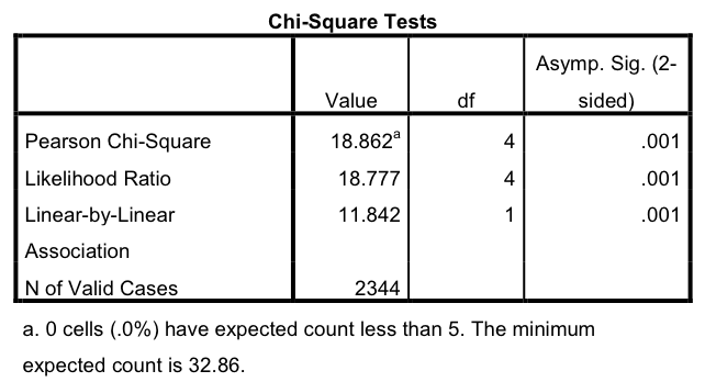
In the following discussion we will sometimes refer to Figure 4.1, which shows SPSS output for the \(\chi^{2}\) test of independence for the data in Table 4.1. Output for the test is shown on the line labelled “Pearson Chi-Square”, and “N of valid cases” gives the sample size \(n\). The other entries in the table are output for other tests that are not discussed here, so they can be ignored.
When we apply any significance test, we need to be aware of its assumptions. These are conditions on the data which are not themselves being tested, but which need to be approximately satisfied for the conclusions from the test to be valid. Two broad types of such assumptions are particularly common. The first kind are assumptions about the measurement levels and population distributions of the variables. For the \(\chi^{2}\) test of independence these are relatively mild. The two variables must be categorical variables. They can have any measurement level, although in most cases this will be either nominal or ordinal. The test makes no use of the ordering of the categories, so it effectively treats all variables as if they were nominal.
The second common class of assumptions are conditions on the sample size. Many significance tests are appropriate only if this is sufficiently large. For the \(\chi^{2}\) test, the expected frequencies \(f_{e}\) (which will be defined below) need to be large enough in every cell of the table. A common rule of thumb is that the test can be safely used if all expected frequencies are at least 5. Another, slightly more lenient rule requires only that no more than 20% of the expected frequencies are less than 5, and that none are less than 1. These conditions can easily be checked with the help of SPSS output for the \(\chi^{2}\) test, as shown in Figure 4.1. This gives information on the number and proportion of expected frequencies (referred to as “expected counts”) less than five, and also the size of the smallest of them. In our example the smallest expected frequency is about 33, so the sample size condition is easily satisfied.
When the expected frequencies do not satisfy these conditions, the \(\chi^{2}\) test is not fully valid, and the results should be treated with caution (the reasons for this will be discussed below). There are alternative tests which do not rely on these large-sample assumptions, but they are beyond the scope of this course.
In general, the hypotheses of a test define the questions it can answer, and its assumptions indicate the types of data it is appropriate for. Different tests have different hypotheses and assumptions, which need to be considered in deciding which test is appropriate for a given analysis. We will introduce a number of different significance tests in this coursepack, and give guidelines for choosing between them.
4.3.3 The test statistic
A test statistic is a number calculated from the sample (i.e. a statistic in the sense defined at the beginning of Section 2.6) which is used to test a null hypothesis. We we will describe the calculation of the \(\chi^{2}\) test statistic step by step, using the data in Table 4.1 for illustration. All of the elements of the test statistic for this example are shown in Table 4.2. These elements are
The observed frequencies, denoted \(f_{o}\), one for each cell of the table. These are simply the observed cell counts (compare the \(f_{o}\) column of Table 4.2 to the counts in Table 4.1).
The expected frequencies \(f_{e}\), also one for each cell. These are cell counts in a hypothetical table which would show no association between the variables. In other words, they represent a table for a sample which would exactly agree with the null hypothesis of independence in the population. To explain how the expected frequencies are calculated, consider the cell in Table 4.1 for Male respondents who strongly agree with the statement. As discussed above, if the null hypothesis of independence is true in the population, then the conditional probability of strongly agreeing is the same for both men and women. This also implies that it must then be equal to the overall (marginal) probability of strongly agreeing. The sample version of this is that the proportion who strongly agree should be the same for men as among all respondents overall. This overall proportion in Table 4.1 is \(366/2344=0.156\). If this proportion applied also to the 1027 male respondents, the number of of them who strongly agreed would be \[f_{e} = \left(\frac{366}{2344}\right)\times 1027 = \frac{366\times 1027}{2344}=160.4.\] Here 2344 is the total sample size, and 366 and 1027 are the marginal frequencies of strongly agreers and male respondents respectively, i.e. the two marginal totals corresponding to the cell (Male, Strongly agree). The same rule applies also in general: the expected frequency for any cell in this or any other table is calculated as the product of the row and column totals corresponding to the cell, divided by the total sample size.
The difference \(f_{o}-f_{e}\) between observed and expected frequencies for each cell. Since \(f_{e}\) are the cell counts in a table which exactly agrees with the null hypothesis, the differences indicate how closely the counts \(f_{o}\) actually observed agree with \(H_{0}\). If the differences are small, the observed data are consistent with the null hypothesis, whereas large differences indicate evidence against it. The test statistic will be obtained by aggregating information about these differences across all the cells of the table. This cannot, however, be done by adding up the differences themselves, because positive (\(f_{o}\) is larger than \(f_{e}\)) and negative (\(f_{o}\) is smaller than \(f_{e}\)) differences will always exactly cancel each other out (c.f. their sum on the last row of Table 4.2). Instead, we consider…
…the squared differences \((f_{o}-f_{e})^{2}\). This removes the signs from the differences, so that the squares of positive and negative differences which are equally far from zero will be treated as equally strong evidence against the null hypothesis.
Dividing the squared differences by the expected frequencies, i.e. \((f_{o}-f_{e})^{2}/f_{e}\). This is an essential but not particularly interesting scaling exercise, which expresses the sizes of the squared differences relative to the sizes of \(f_{e}\) themselves.
Finally, aggregating these quantities to get the \(\chi^{2}\) test statistic \[\begin{equation} \chi^{2} = \sum \frac{(f_{o}-f_{e})^{2}}{f_{e}}. \tag{4.3} \end{equation}\] Here the summation sign \(\Sigma\) indicates that \(\chi^{2}\) is obtained by adding up the quantities \((f_{o}-f_{e})^{2}/f_{e}\) across all the cells of the table.
| Sex | Attitude | \(f_{o}\) | \(f_{e}\) | \(f_{o}-f_{e}\) | \((f_{o}-f_{e})^{2}\) | \((f_{o}-f_{e})^{2}/f_{e}\) |
|---|---|---|---|---|---|---|
| Male | SA | 160 | 160.4 | \(-0.4\) | 0.16 | 0.001 |
| Male | A | 439 | 477.6 | \(-38.6\) | 1489.96 | 3.120 |
| Male | 0 | 187 | 186.6 | 0.4 | 0.16 | 0.001 |
| Male | D | 200 | 169.6 | 30.4 | 924.16 | 5.449 |
| Male | SD | 41 | 32.9 | 8.1 | 65.61 | 1.994 |
| Female | SA | 206 | 205.6 | 0.4 | 0.16 | 0.001 |
| Female | A | 651 | 612.4 | 38.6 | 1489.96 | 2.433 |
| Female | 0 | 239 | 239.4 | \(-0.4\) | 0.16 | 0.001 |
| Female | D | 187 | 217.4 | \(-30.4\) | 924.16 | 4.251 |
| Female | SD | 34 | 42.1 | \(-8.1\) | 65.61 | 1.558 |
| Sum | 2344 | 2344 | 0 | 4960.1 | \(\chi^{2}=18.81\) |
The calculations can be done even by hand, but we will usually leave them to a computer. The last column of Table 4.2 shows that for Table 4.1 the test statistic is \(\chi^{2}=18.81\) (which includes some rounding error, the correct value is 18.862). In the SPSS output in Figure 4.1, it is given in the “Value” column of the “Pearson Chi-Square” row.
4.3.4 The sampling distribution of the test statistic
We now know that the value of the \(\chi^{2}\) test statistic in the example is 18.86. But what does that mean? Why is the test statistic defined as ((4.3)) and not in some other form? And what does the number mean? Is 18.86 small or large, weak or strong evidence against the null hypothesis that sex and attitude are independent in the population?
In general, a test statistic for any null hypothesis should satisfy two requirements:
The value of the test statistic should be small when evidence against the null hypothesis is weak, and large when this evidence is strong.
The sampling distribution of the test statistic should be known and of convenient form when the null hypothesis is true.
Taking the first requirement first, consider the form of ((4.3)). The important part of this are the squared differences \((f_{o}-f_{e})^{2}\) for each cell of the table. Here the expected frequencies \(f_{e}\) reveal what the table would look like if the sample was in perfect agreement with the claim of independence in the population, while the observed frequencies \(f_{o}\) show what the observed table actually does look like. If \(f_{o}\) in a cell is close to \(f_{e}\), the squared difference is small and the cell contributes only a small addition to the test statistic. If \(f_{o}\) is very different from \(f_{e}\) — either much smaller or much larger than it — the squared difference and hence the cell’s contribution to the test statistic are large.
Summing the contributions over all the cells, this implies that the overall value of the test statistic is small when the observed frequencies are close to the expected frequencies under the null hypothesis, and large when at least some of the observed frequencies are far from the expected ones. (Note also that the smallest possible value of the statistic is 0, obtained when the observed and the expected frequency are exactly equal in each cell.) It is thus large values of \(\chi^{2}\) which should be regarded as evidence against the null hypothesis, just as required by condition 1 above.
Turning then to condition 2, we first need to explain what is meant by “sampling distribution of the test statistic … when the null hypothesis is true”. This is really the conceptual crux of significance testing. Because it is both so important and relatively abstract, we will introduce the concept of a sampling distribution in some detail, starting with a general definition and then focusing on the case of test statistics in general and the \(\chi^{2}\) test in particular.
Sampling distribution of statistic: General definition
The \(\chi^{2}\) test statistic ((4.3)) is a statistic as defined defined at the beginning of Section 2.6, that is a number calculated from data in a sample. Once we have observed a sample, the value of a statistic in that sample is known, such as the 18.862 for \(\chi^{2}\) in our example.
However, we also realise that this value would have been different if the sample had been different, and also that the sample could indeed have been different because the sampling is a process that involves randomness. For example, in the actually observed sample in Table 4.1 we had 200 men who disagreed with the statement and 41 who strongly disagreed with it. It is easily imaginable that another random sample of 2344 respondents from the same population could have given us frequencies of, say, 195 and 46 for these cells instead. If that had happened, the value of the \(\chi^{2}\) statistic would have been 19.75 instead of 18.86. Furthermore, it also seems intuitively plausible that not all such alternative values are equally likely for samples from a given population. For example, it seems quite improbable that the population from which the sample in Table 4.1 was drawn would instead produce a sample which also had 1027 men and 1317 women but where all the men strongly disagreed with the statement (which would yield \(\chi^{2}=2210.3\)).
The ideas that different possible samples would give different values of a sample statistic, and that some such values are more likely than others, are formalised in the concept of a sampling distribution:
- The sampling distribution of a statistic is the distribution of the statistic (i.e. its possible values and the proportions with which they occur) in the set of all possible random samples of the same size from the population.
To observe a sampling distribution of a statistic, we would thus need to draw samples from the population over and over again, and calculate the value of the statistic for each such sample, until we had a good idea of the proportions with which different values of the statistic appeared in the samples. This is clearly an entirely hypothetical exercise in most real examples where we have just one sample of actual data, whereas the number of possible samples of that size is essentially or actually infinite. Despite this, statisticians can find out what sampling distributions would look like, under specific assumptions about the population. One way to do so is through mathematical derivations. Another is a computer simulation where we use a computer program to draw a large number of samples from an artificial population, calculate the value of a statistic for each of them, and examine the distribution of the statistic across these repeated samples. We will make use of both of these approaches below.
Sampling distribution of a test statistic under the null hypothesis
The sampling distribution of any statistic depends primarily on what the population is like. For test statistics, note that requirement 2 above mentioned only the situation where the null hypothesis is true. This is in fact the central conceptual ingredient of significance testing. The basic logic of drawing conclusions from such tests is that we consider what we would expect to see if the null hypothesis was in fact true in the population, and compare that to what was actually observed in our sample. The null hypothesis should then be rejected if the observed data would be surprising (i.e. unlikely) if the null hypothesis was actually true, and not rejected if the observed data would not be surprising under the null hypothesis.
We have already seen that the \(\chi^{2}\) test statistic is in effect a measure of the discrepancy between what is expected under the null hypothesis and what is observed in the sample. All test statistics for any hypotheses have this property in one way or another. What then remains to be determined is exactly how surprising or otherwise the observed data are relative to the null hypothesis. A measure of this is derived from the sampling distribution of the test statistic under the null hypothesis. It is the only sampling distribution that is needed for carrying out a significance test.
Sampling distribution of the \(\chi^{2}\) test statistic under independence
For the \(\chi^{2}\) test, we need the sampling distribution of the test statistic ((4.3)) under the independence null hypothesis ((4.1)). To make these ideas a little more concrete, the upper part of Table 4.3 shows the crosstabulation of sex and attitude in our example for a finite population where the null hypothesis holds. We can see that it does because the two conditional distributions for attitude, among men and among women, are the same (this is the only aspect of the distributions that matters for this demonstration; the exact values of the probabilities are otherwise irrelevant). These are of course hypothetical population distributions, as we do not know the true ones. We also do not claim that this hypothetical population is even close to the true one. The whole point of this step of hypothesis testing is to set up a population where the null hypothesis holds as a fixed point of comparison, to see what samples from such a population would look like and how they compare with the real sample that we have actually observed.
Population (frequencies are in millions of people):
|
Sex |
Agree strongly |
Agree |
Neither agree nor disagree |
Disagree |
Disagree strongly |
Total |
|---|---|---|---|---|---|---|
| Male | 3.744 | 11.160 | 4.368 | 3.960 | 0.768 | 24.00 |
| (0.156) | (0.465) | (0.182) | (0.165) | (0.032) | (1.0) | |
| Female | 4.056 | 12.090 | 4.732 | 4.290 | 0.832 | 26.00 |
| (0.156) | (0.465) | (0.182) | (0.165) | (0.032) | (1.0) | |
| Total | 7.800 | 23.250 | 9.100 | 8.250 | 1.600 | 50 |
| (0.156) | (0.465) | (0.182) | (0.165) | (0.032) | (1.0) |
Sample:
|
Sex |
Agree strongly |
Agree |
Neither agree nor disagree |
Disagree |
Disagree strongly |
Total |
|---|---|---|---|---|---|---|
| Male | 181 | 505 | 191 | 203 | 41 | 1121 |
| (0.161) | (0.450) | (0.170) | (0.181) | (0.037) | (1.0) | |
| Female | 183 | 569 | 229 | 202 | 40 | 1223 |
| (0.150) | (0.465) | (0.187) | (0.165) | (0.033) | (1.0) | |
| Total | 364 | 1074 | 420 | 405 | 81 | 2344 |
| (0.155) | (0.458) | (0.179) | (0.173) | (0.035) | (1.0) |
In the example we have a sample of 2344 observations, so to match that we want to identify the sampling distribution of the \(\chi^{2}\) statistic in random samples of size 2344 from the population like the one in the upper part of Table 4.3. The lower part of that table shows one such sample. Even though it comes from a population where the two variables are independent, the same is not exactly true in the sample: we can see that the conditional sample distributions are not the same for men and women. The value of the \(\chi^{2}\) test statistic for this simulated sample is 2.8445.
Before we proceed with the discussion of the sampling distribution of the \(\chi^{2}\) statistic, we should note that it will be a continuous probability distribution. In other words, the number of distinct values that the test statistic can have in different samples is so large that their distribution is clearly effectively continuous. This is true even though the two variables in the contingency table are themselves categorical. The two distributions, the population distribution of the variables and the sampling distribution of a test statistic, are quite separate entities and need not resemble each other. We will consider the nature of continuous probability distributions in more detail in Chapter 7. In this chapter we will discuss them relatively superficially and only to the extent that is absolutely necessary.
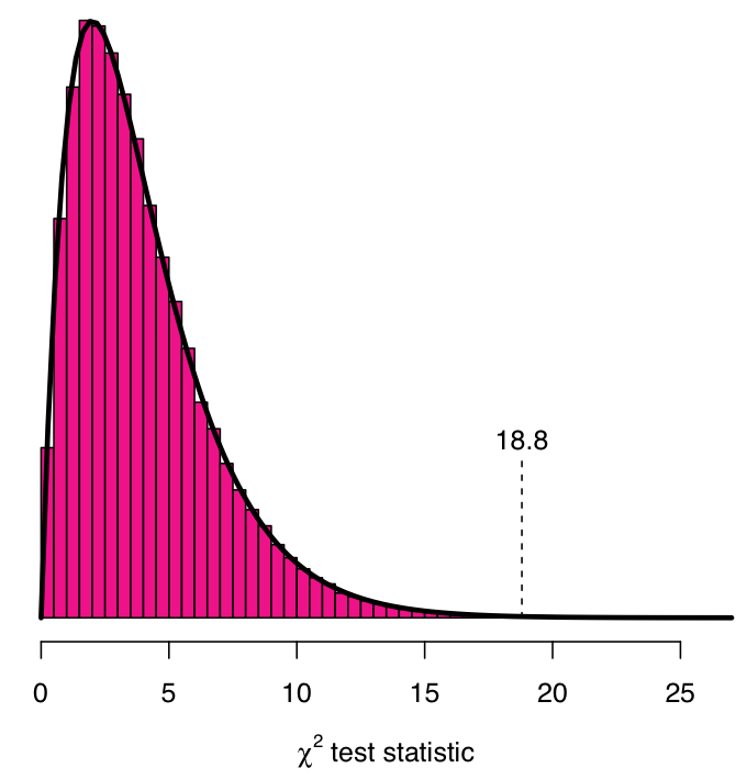
Figure 4.2 shows what we observe if do a computer simulation to draw many more samples from the population in Table 4.3. The figure shows the histogram of the values of the \(\chi^{2}\) test statistic calculated from 100,000 such samples. We can see, for example, that \(\chi^{2}\) is between 0 and 10 for most of the samples, and larger than that for only a small proportion of them. In particular, we note already that the value \(\chi^{2}=18.8\) that was actually observed in the real sample occurs very rarely if samples are drawn from a population where the null hypothesis of independence holds.
The form of the sampling distribution can also be derived through mathematical arguments. These show that for any two-way contingency table, the approximate sampling distribution of the \(\chi^{2}\) statistic is a member of a class of continuous probability distributions known as the \(\boldsymbol{\chi}^{2}\) distributions (the same symbol \(\chi^{2}\) is rather confusingly used to refer both to the test statistic and its sampling distribution). The \(\chi^{2}\) distributions are a family of individual distributions, each of which is identified by a number known as the degrees of freedom of the distribution. Figure 4.3 shows the probability curves of some \(\chi^{2}\) distributions (what such curves mean is explained in more detail below, and in Chapter 7). All of the distributions are skewed to the right, and the shape of a particular curve depends on its degrees of feedom. All of the curves give non-zero probabilites only for positive values of the variable on the horizontal axis, indicating that the value of a \(\chi^{2}\)-distributed variable can never be negative. This is appropriate for the \(\chi^{2}\) test statistic ((4.3)), which is also always non-negative.

For the \(\chi^{2}\) test statistic of independence we have the following result:
- When the null hypothesis ((4.1)) is true in the population, the sampling distribution of the test statistic ((4.3)) calculated for a two-way table with \(R\) rows and \(C\) columns is approximately the \(\chi^{2}\) distribution with \(df=(R-1)(C-1)\) degrees of freedom.
The degrees of freedom are thus given by the number of rows in the table minus one, multiplied by the number of columns minus one. Table 4.1, for example, has \(R=2\) rows and \(C=5\) columns, so its degrees of freedom are \(df=(2-1)\times(5-1)=4\) (as indicated by the “df” column of the SPSS output of Figure 4.1). Figure 4.2 shows the curve of the \(\chi^{2}\) distribution with \(df=4\) superimposed on the histogram of the sampling distribution obtained from the computer simulation. The two are in essentially perfect agreement, as mathematical theory indicates they should be.
These degrees of freedom can be given a further interpretation which relates to the structure of the table.16 We can, however, ignore this and treat \(df\) simply as a number which identifies the appropriate \(\chi^{2}\) distribution to be used for the \(\chi^{2}\) test for a particular table. Often it is convenient to use the notation \(\chi^{2}_{df}\) to refer to a specific distribution, e.g. \(\chi^{2}_{4}\) for the \(\chi^{2}\) distribution with 4 degrees of freedom.
The \(\chi^{2}\) sampling distribution is “approximate” in that it is an asymptotic approximation which is exactly correct only if the sample size is infinite and approximately correct when it is sufficiently large. This is the reason for the conditions for the sizes of the expected frequencies that were discussed in Section 4.3.2. When these conditions are satisfied, the approximation is accurate enough for all practical purposes and we use the appropriate \(\chi^{2}\) distribution as the sampling distribution.
In Section 4.3.4, under requirement 2 for a good test statistic, we mentioned that its sampling distribution under the null hypothesis should be “known” and “of convenient form”. We now know that for the \(\chi^{2}\) test it is a \(\chi^{2}\) distribution. The “convenient form” means that the sampling distribution should not depend on too many specific features of the data at hand. For the \(\chi^{2}\) test, the approximate sampling distribution depends (through the degrees of freedom) only on the size of the table but not on the sample size or the marginal distributions of the two variables. This is convenient in the right way, because it means that we can use the same \(\chi^{2}\) distribution for any table with a given number of rows and columns, as long as the sample size is large enough for the conditions in Section 4.3.2 to be satisfied.
4.3.5 The P-value
The last key building block of significance testing operationalises the comparison between the observed value of a test statistic and its sampling distribution under the null hypothesis. In essence, it provides a way to determine whether the test statistic in the sample should be regarded as “large” or “not large”, and with this the measure of evidence against the null hypothesis that is the end product of the test:
- The \(\mathbf{P}\)-value is the probability, if the null hypothesis was true in the population, of obtaining a value of the test statistic which provides as strong or stronger evidence against the null hypothesis, and in the direction of the alternative hypothesis, as the the value of the test statistic in the sample actually observed.
The relevance of the phrase “in the direction of the alternative hypothesis” is not apparent for the \(\chi^{2}\) test, so we can ignore it for the moment. As argued above, for this test it is large values of the test statistic which indicate evidence against the null hypothesis of independence, so the values that correspond to “as strong or stronger evidence” against it are the ones that are as large or larger than the observed statistic. Their probability is evaluated from the \(\chi^{2}\) sampling distribution defined above.
Figure 4.4 illustrates this calculation. It shows the curve of the \(\chi^{2}_{4}\) distribution, which is the relevant sampling distribution for the test for the \(2\times 5\) table in our example. Suppose first, hypothetically, that we had actually observed the sample in the lower part of Table 4.3, for which the value of the test statistic is \(\chi^{2}=2.84\). The \(P\)-value of the test for this sample would then be the probability of values of 2.84 or larger, evaluated from the \(\chi^{2}_{4}\) distribution.
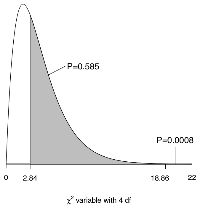
For a probability curve like the one in Figure 4.4, areas under the curve correspond to probabilities. For example, the area under the whole curve from 0 to infinity is 1, because a variable which follows the \(\chi^{2}_{4}\) distribution is certain to have one of these values. Similarly, the probability that we need for the \(P\)-value for \(\chi^{2}=2.84\) is the area under the curve to the right of the value 2.84, which is shown in grey in Figure 4.4. This is \(P=0.585\).
The test statistic for the real sample in Table 4.1 was \(\chi^{2}=18.86\), so the \(P\)-value is the combined probability of this and all larger values. This is also shown in Figure 4.4. However, this area is not really visible in the plot because 18.86 is far into the tail of the distribution where the probabilities are low. The \(P\)-value is then also low, specifically \(P=0.0008\).
In practice the \(P\)-value is usually calculated by a computer. In the SPSS output of Figure 4.1 is is shown in the column labelled “Asymp. Sig. (2-sided)” which is short for “Asymptotic significance level” (you can ignore the “2-sided” for this test). The value is listed as 0.001. SPSS reports, by default, \(P\)-values rounded to three decimal places. Sometimes even the smallest of these is zero, in which case the value is displayed as “.000”. This is bad practice, as the \(P\)-value for most significance tests is never exactly zero. \(P\)-values given by SPSS as “.000” should be reported instead as “\(P<0.001\)”.
Before the widespread availablity of statistical software, \(P\)-values had to be obtained approximately using tables of distributions. Since you may still see this approach described in many text books, it is briefly explained here. You may also need to use the table method in the examination, where computers are not allowed. Otherwise, however, this approach is now of little interest: if the \(P\)-value is given in the computer output, there is no need to refer to distributional tables.
All introductory statistical text books include a table of \(\chi^{2}\) distributions, although its format may vary slightly form book to book. Such a table is also included in the Appendix of this coursepack. An extract from the table is shown in Table 4.4. Each row of the table corresponds to a \(\chi^{2}\) distribution with the degrees of freedom given in the first column. The other columns show so-called “critical values” for the probability levels given on the first row. Consider, for example, the row for 4 degrees of freedom. The figure 7.78 in the column for probability level 0.100 indicates that the probability of a value of 7.78 or larger is exactly 0.100 for this distribution. The 9.49 in the next column shows that the probability of 9.49 or larger is 0.050. Another way of saying this is that if the appropriate degrees of freedom were 4, and the test statistic was 7.78, the \(P\)-value would be exactly 0.100, and if the statistic was 9.49, \(P\) would be 0.050.
| df | 0.100 | 0.050 | 0.010 | 0.001 |
|---|---|---|---|---|
| 1 | 2.71 | 3.84 | 6.63 | 10.83 |
| 2 | 4.61 | 5.99 | 9.21 | 13.82 |
| 3 | 6.25 | 7.81 | 11.34 | 16.27 |
| 4 | 7.78 | 9.49 | 13.28 | 18.47 |
| … | … | … |
The values in the table also provide bounds for other values that are not shown. For instance, in the hypothetical sample in Table 4.3 we had \(\chi^{2}=2.84\), which is smaller than 7.78. This implies that the corresponding \(P\)-value must be larger than 0.100, which (of course) agrees with the precise value of \(P=0.585\) (see also Figure 4.4). Similarly, \(\chi^{2}=18.86\) for the real data in Table 4.1, which is larger than the 18.47 in the “0.001” column of the table for the \(\chi^{2}_{4}\) distribution. Thus the corresponding \(P\)-value must be smaller than 0.001, again agreeing with the correct value of \(P=0.0008\).
4.3.6 Drawing conclusions from a test
The \(P\)-value is the end product of any significance test, in that it is a complete quantitative summary of the strength of evidence against the null hypothesis provided by the data in the sample. More precisely, the \(P\)-value indicates how likely we would be to obtain a value of the test statistic which was as or more extreme as the value for the data, if the null hypothesis was true. Thus the smaller the \(P\)-value, the stronger is the evidence against the null hypothesis. For example, in our survey example of sex and attitude toward income redistribution we obtained \(P=0.0008\) for the \(\chi^{2}\) test of independence. This is a small number, so it indicates strong evidence against the claim that the distributions of attitudes are the same for men and women in the population.
For many purposes it is quite sufficient to simply report the \(P\)-value. It is, however, quite common also to state the conclusion in the form of a more discrete decision of “rejecting” or “not rejecting” the null hypothesis. This is usually based on conventional reference levels, known as significance levels or \(\boldsymbol{\alpha}\)-levels (here \(\alpha\) is the lower-case Greek letter “alpha”). The standard significance levels are 0.10, 0.05, 0.01 and 0.001 (also known as 10%, 5%, 1% and 0.1% significance levels respectively), of which the 0.05 level is most commonly used; other values than these are rarely considered. The values of the test statistic which correspond exactly to these levels are the critical shown in the table of the \(\chi^{2}\) distribution in Table 4.4.
When the \(P\)-value is smaller than a conventional level of significance (i.e. the test statistic is larger than the corresponding critical value), it is said that the null hypothesis is rejected at that level of significance, or that the results (i.e. evidence against the null hypothesis) are statistically significant at that level. In our example the \(P\)-value was smaller than 0.001. The null hypothesis is thus “rejected at the 0.1 % level of significance”, i.e. the evidence that the variables are not independent in the population is “statistically significant at the 0.1% level” (as well as the 10%, 5% and 1% levels of course, but it is enough to state only the strongest level).
The strict decision formulation of significance testing is much overused and misused. It is in fact quite rare that the statistical analysis will immediately be followed by some practical action which absolutely requires a decision about whether to act on the basis of the null hypothesis or the alternative hypothesis. Typically the analysis which a test is part of aims to examine some research question, and the results of the test simply contribute new information to add support for one or the other side of the argument about the question. The \(P\)-value is the key measure of the strength and direction of that evidence, so it should always be reported. The standard significance levels used for rejecting or not rejecting null hypotheses, on the other hand, are merely useful conventional reference points for structuring the reporting of test results, and their importance should not be overemphasised. Clearly \(P\)-values of, say, 0.049 and 0.051 (i.e. ones either side of the most common conventional significance level 0.05) indicate very similar levels of evidence against a null hypothesis, and acting as if one was somehow qualitatively more decisive is simply misleading.
How to state the conclusions
The final step of a significance test is describing its conclusions in a research report. This should be done with appropriate care:
The report should make clear which test was used. For example, this might be stated as something like “The \(\chi^{2}\) test of independence was used to test the null hypothesis that in the population the attitude toward income redistribution was independent of sex in the population”. There is usually no need to give literature references for the standard tests described on this course.
The numerical value of the \(P\)-value should be reported, rounded to two or three decimal places (e.g. \(P=0.108\) or \(P=0.11\)). It can also reported in an approximate way as, for example, “\(P<0.05\)” (or the same in symbols to save space, e.g. for \(P<0.1\), ** for \(P<0.05\), and so on). Very small \(P\)-values can always be reported as something like “\(P<0.001\)”.
When (cautiously) discussing the results in terms of discrete decisions, the most common practice is to say that the null hypothesis was either not rejected or rejected at a given significance level. It is not acceptable to say that the null hypothesis was “accepted” as an alternative to “not rejected”. Failing to reject the hypothesis that two variables are independent in the population is not the same as proving that they actually are independent.
A common mistake is to describe the \(P\)-value as the probability that the null hypothesis is true. This is understandably tempting, as such a claim would seem more natural and convenient than the correct but convoluted interpretation of the \(P\)-value as “the probability of obtaining a test statistic as or more extreme as the one observed in the data if the test was repeated many times for different samples from a population where the null hypothesis was true”. Unfortunately, however, the \(P\)-value is not the probability of the null hypothesis being true. Such a probability does not in fact have any real meaning at all in the statistical framework considered here.17
-
The results of significance tests should be stated using the names and values of the variables involved, and not just in terms of “null” and “alternative” hypotheses. This also forces you to recall what the hypotheses actually were, so that you do not accidentally describe the result the wrong way round (e.g. that the data support a claim when they do just the opposite). There are no compulsory phrases for stating the conclusions, so it can be done in a number of ways. For example, a fairly complete and careful statement in our example would be
- “There is strong evidence that the distributions of attitudes toward income redistribution are not the same for men and women in the population (\(P<0.001\)).”
Other possibilities are
“The association between sex and attitude toward income redistribution in the sample is statistically significant (\(P<0.001\)).”
“The analysis suggests that there is an association between sex and attitude toward income redistribution in the population (\(P<0.001\)).”
The last version is slightly less clear than the other statements in that it relies on the reader recognizing that the inclusion of the \(P\)-value implies that the word “differs” refers to a statistical claim rather a statement of absolute fact about the population. In many contexts it would be better to say this more explicitly.
Finally, if the null hypothesis of independence is rejected, the test should not usually be the only statistical analysis that is reported for a two-way table. Instead, we would then go on to describe how the two variables appear to be associated, using the of descriptive methods discussed in Section 2.4.
4.4 Summary of the chi-square test of independence
We have now described the elements of a significance test in some detail. Since it is easy to lose sight of the practical steps of a test in such a lengthy discussion, they are briefly repeated here for the \(\chi^{2}\) test of independence. The test of the association between sex and attitude in the survey example is again used for illustration:
Data: observations of two categorical variables, here sex and attitude towards income redistribution for \(n=2344\) respondents, presented in the two-way, \(2\times 5\) contingency table 4.1.
Assumptions: the variables can have any measurement level, but the expected frequencies \(f_{e}\) must be large enough. A common rule of thumb is that \(f_{e}\) should be at least 5 for every cell of the table. Here the smallest expected frequency is 32.9, so the requirement is comfortably satisfied.
Hypotheses: null hypothesis \(H_{0}\) that the two variables are statistically independent (i.e. not associated) in the population, against the alternative hypothesis that they are dependent.
The test statistic: the \(\chi^{2}\) statistic \[\chi^{2} = \sum \frac{(f_{o}-f_{e})^{2}}{f_{e}}\] where \(f_{o}\) denotes observed frequencies in the cells of the table and \(f_{e}\) the corresponding expected frequencies under the null hypothesis, and the summation is over all of the cells. For Table 4.1, \(\chi^{2}=18.86\).
The sampling distribution of the test statistic when \(H_{0}\) is true: a \(\chi^{2}\) distribution with \((R-1)\times(C-1)=1\times 4=4\) degrees of freedom, where \(R\) \((=2)\) and \(C\) \((=5)\) denote the numbers of rows and columns in the table respectively.
The \(P\)-value: the probability that a randomly selected value from the \(\chi^{2}_{4}\) distribution is at least 18.86. This is \(P=0.0008\), which may also be reported as \(P<0.001\).
Conclusion: the null hypothesis of independence is strongly rejected. The \(\chi^{2}\) test indicates very strong evidence that sex and attitude towards income redistribution are associated in the population (\(P<0.001\)).
When the association is judged to be statistically significant, its nature and magnitude can be further explored using the descriptive methods for two way tables discussed in Section 2.4.