5 Inference for population proportions
5.1 Introduction
In this chapter we still consider statistical analyses which involve only discrete, categorical variables. In fact, we now focus on the simplest case of all, that of dichotomous (binary) variables which have only two possible values. Four examples which will be used for illustration throughout this chapter are introduced in Section 5.2. In the first two of them we consider a binary variable in a single population, while in the last two examples the question of interest involves a comparison of the distributions of the variable between two populations (groups).
The data for such analyses can be summarised in simple tables, the one-group case with a one-way table of two cells, and the two-group case with a \(2\times 2\) contingency table. Here, however, we formulate the questions of interest slightly differently, with primary emphasis on the probability of one of the two values of the variable of interest. In the one-group case the questions of interest are then about the population value of a single probability, and in the two-group case about the comparison of the values of this probability between the two groups.
While we describe specific methods of inference for these cases, we also use them to introduce some further general elements of statistical inference:
Population parameters of probability distributions.
Point estimation of population parameters.
Hypotheses anout the parameters, and significance tests for them.
Confidence intervals for population parameters.
The comparisons in the two-group analyses again address questions about associations, now between the group and the dichotomous variable of interest. Here it will be useful to employ the terminology introduced in Section 1.2.4, which distinguishes between the explanatory variable and the response variable in the association. Following a common convention, we will denote the explanatory variable by \(X\) and the response variable by \(Y\). In the two-group cases of this chapter, \(X\) will be the group (which is itself also binary) and \(Y\) the binary variable whose probabilities we are interested in. We will use \(Y\) to denote this binary variable also in the one-group examples.
5.2 Examples
The following four examples will be discussed in this chapter. Examples 5.1 and 5.2 concern only one group, while in Examples 5.3 and 5.4 two groups are to be compared. Table 5.1 shows basic sample statistics for the examples, together with the results of the significance tests and confidence intervals described later.
Example 5.1: An EU referendum
A referendum about joining the European Union was held in Finland on the 16th of October, 1994. Suppose that in an opinion poll conducted around October 4th (just before the beginning of postal voting), 330 of the \(n=702\) respondents (47.0%) indicated that they would definitely vote Yes to joining the EU, 190 (27.1%) said they would definitely vote No, and 182 (25.9%) were still undecided.18 Here we will consider the dichotomous variable with the values of Yes (330 respondents) versus No or Undecided (372 respondents, or 53.0%). The proportion of voters who definitely intend to vote Yes provides a lower bound for the proportion of Yes-votes in the referendum, even if all of the currently undecided voters eventually decided to vote No.
Example 5.2: Evidence of possible racial bias in jury selection
As part of an official inquiry into the extent of racial and gender bias in the justice system in the U.S. state of Pennsylvania, an investigation was made of whether people from minority racial groups were underrepresented in trial juries.19 One part of the assessment was a survey administered to all those called for the jury panel for criminal trials (from which the juries for actual trials will be selected) in Allegheny County, Pennsylvania (the city of Pittsburgh and its surrounding areas) between May and October, 2001. We will consider the dichotomous variable of whether a respondent to the survey identified his or her own race as Black (African American) or some other race category. Of the \(n=4950\) respondents, 226 (4.57%) identified themselves as black. This will be compared to the the percentage of black people in the whole population of people aged 18 and over (those eligible for jury service) in the county, which is 12.4% (this is a census estimate which will here be treated as a known population quantity, ignoring any possible census error in it).
| One sample | |||||||
| Example 5.1: Voting intention in an EU referendum | |||||||
| \(n\) | Yes | \(\hat{\pi}\) | \(\pi_{0}\) | \(z\) | \(P\) | 95% CI | |
| 702 | 330 | 0.470 | 0.5 | \(-1.59\) | 0.112 | (0.433; 0.507) | |
| Example 5.2: Race of members of jury panel | |||||||
| \(n\) | Black | \(\hat{\pi}\) | \(\pi_{0}\) | \(z\) | \(P\) | 95% CI | |
| 4950 | 226 | 0.0457 | 0.124 | \(-16.71\) | \(<0.001\) | (0.040; 0.052) | |
| Two Independent samples | |||||||
| Example 5.3: Polio diagnoses in a vaccine trial | |||||||
| \(n\) | Yes | \(\hat{\pi}\) | Diff. (\(\hat{\Delta}\)) | \(z\) | \(P\) | 95% CI | |
| Control group (placebo) | 201,229 | 142 | 0.000706 | ||||
| Treatment group (vaccine) | 200,745 | 57 | 0.000284 | \(-0.000422\) | \(-6.01\) | \(<0.001\) | \((-0.000560;\) \(-0.000284)\) |
| Example 5.4: Optimistic about young people’s future | |||||||
| \(n\) | Yes | \(\hat{\pi}\) | Diff. (\(\hat{\Delta}\)) | \(z\) | \(P\) | 95% CI | |
| Negative question | 921 | 257 | 0.279 | ||||
| Positive question | 929 | 338 | 0.364 | 0.085 | 3.92 | \(<0.001\) | (0.043; 0.127) |
Example 5.3: The Salk polio vaccine field trial of 1954
The first large-scale field trials of the “killed virus” polio vaccination developed by Dr. Jonas Salk were carried out in the U.S. in 1954.20 In the randomized, double-blind placebo-control part of the trial, a sample of schoolchildren were randomly assigned to receive either three injections of the polio vaccine, or three injections of a placebo, inert saltwater which was externally indistinguishable from the real vaccine. The explanatory variable \(X\) is thus the group (vaccine or “treatment” group vs. placebo or “control” group). The response variable \(Y\) is whether the child was diagnosed with polio during the trial period (yes or no). There were \(n_{1}=201,229\) children in the control group, and 142 of them were diagnosed with polio; in the treatment group, there were 57 new polio cases among \(n_{2}=200,745\) children (in both cases only those children who received all three injections are included here). The proportions of cases of polio were thus \(0.000706\) in the control group and \(0.000284\) in the vaccinated group (i.e. 7.06 and 2.84 cases per 10,000 subjects, respectively).
Example 5.4: Split-ballot experiment on acquiescence bias
Survey questions often ask whether respondents agree or disagree with given statements on opinions or attitudes. Acquiescence bias means the tendency of respondents to agree with such statements, regardless of their contents. If it is present, we will overestimate the proportion of people holding the opinion corresponding to agreement with the statement. The data used in this example come from a study which examined acquiescence bias through a randomized experiment.21 In a survey carried out in Kazakhstan, the respondents were presented with a number of attitude statements, with four response categories: “Fully agree”, “Somewhat agree”, “Somewhat disagree”, and “Fully disagree”. Here we combine the first two and the last two, and consider the resulting dichotomous variable, with values labelled “Agree” and “Disagree”.
We consider one item from the survey, concerning the respondents’ opinions on the expectations of today’s young people. There were two forms of the question:
“A young person today can expect little of the future”
“A young person today can expect much of the future”
We will call these the “Negative” and “Positive” question respectively. Around half of the respondents were randomly assigned to receive the positive question, and the rest got the negative question. The explanatory variable \(X\) indicates the type of question, with Negative and Positive questions coded here as 1 and 2 respectively. The dichotomous response variable \(Y\) is whether the respondent gave a response which was optimistic about the future (i.e. agreed with the positive or disagreed with the negative question) or a pessimistic response. The sample sizes and proportions of optimistic responses in the two groups are reported in Table 5.1. The proportion is higher when the question was worded positively, as we would expect if there was acquiescence bias. Whether this difference is statistically significant remains to be determined.
5.3 Probability distribution of a dichotomous variable
The response variables \(Y\) considered in this section have only two possible values. It is common to code them as 0 and 1. In our examples, we will define the values of the variable of interest as follows:
Example 5.1: 1 if a person says that he or she will definitely vote Yes, and 0 if the respondent will vote No or is undecided
Example 5.2: 1 for black respondents and 0 for all others
Example 5.3: 1 if a child developed polio, 0 if not
Example 5.4: 1 if the respondent gave an optimistic response, 0 if not
The population distribution of such a variable is completely specified by one number, the probability that a randomly selected member of the population will have the value \(Y=1\) rather than 0. It can also be thought of as the proportion of units in the population with \(Y=1\); we will use the two terms interchangeably. This probability is denoted here \(\pi\) (the lower-case Greek letter “pi”).22 The value of \(\pi\) is between 0 (no-one in the population has \(Y=1\)) and 1 (everyone has \(Y=1\)). Because \(Y\) can have only two possible values, and the sum of probabilities must be one, the population probability of \(Y=0\) is \(1-\pi\).
The probability distribution which corresponds to this kind of population distribution is the Binomial distribution. For later use, we note already here that the mean of this distribution is \(\pi\) and its variance is \(\pi(1-\pi)\).
In Example 5.1, the population is that of eligible voters at the time of the opinion poll, and \(\pi\) is the probability that a randomly selected eligible voter definitely intended to vote Yes. In Example 5.2, \(\pi\) is the probability that a black person living in the county will be selected to the jury panel. In Example 5.3, \(\pi\) is the probability (possibly different in the vaccinated and unvaccinated groups) that a child will develop polio, and in Example 5.4 it is the probability (which possibly depends on how the question was asked) that a respondent will give an optimistic answer to the survey question.
The probability \(\pi\) is the parameter of the binomial distribution. In general, the parameters of a probability distribution are one or more numbers which fully determine the distribution. For example, in the analyses of Chapter 4 we considered conditional distributions of a one variable in a contingency table given the other variable. Although we did not make use of this terminology there, these distributions also have their parameters, whcih are the probabilities of (all but one of) the categories of the response variable. Another case will be introduced in Chapter 7, where we consider a probability distribution for a continuous variable, and its parameters.
5.4 Point estimation of a population probability
Questions and hypotheses about population distributions are usually most conveniently formulated in terms of the parameters of the distributions. For a binary variable \(Y\), this means that statistical inference will be focused on the probability \(\pi\).
The most obvious question about a parameter is “what is our best guess of the value of the parameter in the population?” The answer will be based on the information in the sample, using some sample statistic as the best guess or estimate of the population parameter. Specifically, this is a point estimate, because it is expressed as a single value or a “point”, to distinguish it from interval estimates defined later.
We denote a point estimate of \(\pi\) by \(\hat{\pi}\). The “\(\; \hat{\;}\;\)” or “hat” is often used to denote an estimate of a parameter indicated by the symbol under the hat; \(\hat{\pi}\) is read as “pi-hat”. As \(\pi\) for a binomial distribution is the population proportion of \(Y=1\), the obvious choice for a point estimate of it is the sample proportion of units with \(Y=1\). If we denote the number of such units by \(m\), the proportion is thus \(\hat{\pi}=m/n\), i.e. \(m\) divided by the sample size \(n\). In Example 5.1, \(m=330\) and \(n=702\), and \(\hat{\pi}=330/702=0.47\). This and the estimated proportions in the other examples are shown in Table 5.1, in the two-sample examples 5.3 and 5.4 separately for the two groups.
When \(Y\) is coded with values 0 and 1, \(\hat{\pi}\) is also equal to the sample mean of \(Y\), since \[\begin{equation} \bar{Y}=\frac{Y_{1}+Y_{2}+\dots+Y_{n}}{n}=\frac{0+0+\dots+0+\overbrace{1+1+\dots+1}^{m \text{ ones}}}{n}=\frac{m}{n}=\hat{\pi}. \tag{5.1} \end{equation}\]
5.5 Significance test of a single proportion
5.5.1 Null and alternative hypotheses
A null hypothesis about a single population probability \(\pi\) is of the form \[\begin{equation} H_{0}:\; \pi=\pi_{0} \tag{5.2} \end{equation}\] where \(\pi_{0}\) is a given number which is either of specific interest or in some other sense a suitable benchmark in a given application. For example, in the voting example 5.1 we could consider \(\pi_{0}=0.5\), i.e. that the referendum was too close to call. In the jury example 5.2 the value of interest would be \(\pi_{0}=0.124\), the proportion of black people in the general adult population of the county.
An alternative but equivalent form of ((5.2)) is expressed in terms of the difference \[\begin{equation} \Delta=\pi-\pi_{0} \tag{5.3} \end{equation}\] (\(\Delta\) is the upper-case Greek letter “Delta”). Then (@(5.2)) can also be written as \[\begin{equation} H_{0}: \; \Delta=0, \tag{5.4} \end{equation}\] i.e. that there is no difference between the true population probability and the hypothesised value \(\pi_{0}\). This version of the notation allows us later to draw attention to the similarities between different analyses in this chapter and in Chapter 7. In all of these cases the quantities of interest turn out to be differences of some kind, and the formulas for test statistics and confidence intervals will be of essentially the same form.
The alternative hypothesis to the null hypothesis ((5.4)) requires some further comments, because there are some new possibilities that did not arise for the \(\chi^{2}\) test of independence in Chapter 4. For the difference \(\Delta\), we may consider two basic kinds of alternative hypotheses. The first is a two-sided alternative hypothesis \[\begin{equation} H_{a}: \; \Delta\ne 0 \tag{5.5} \end{equation}\] (where “\(\ne\)” means “not equal to”). This claims that the true value of the population difference \(\Delta\) is some unknown value which is not 0 as claimed by the null hypothesis. With a two-sided \(H_{a}\), sample evidence that the true difference differs from 0 will be regarded as evidence against the null hypothesis, irrespective of whether it suggests that \(\Delta\) is actually smaller or larger than 0 (hence the word “two-sided”). When \(\Delta=\pi-\pi_{0}\), this means that we are trying to assess whether the true probability \(\pi\) is different from the claimed value \(\pi_{0}\), but without any expectations about whether \(\pi\) might be smaller or larger than \(\pi_{0}\).
The second main possibility is one of the two one-sided alternative hypotheses \[\begin{equation} H_{a}: \Delta> 0 \tag{5.6} \end{equation}\] or \[\begin{equation} H_{a}: \Delta < 0 \tag{5.7} \end{equation}\] Such a hypothesis is only interested in values of \(\Delta\) to one side of 0, either larger or smaller than it. For example, hypothesis ((5.6)) in the referendum example 5.1, with \(\pi_{0}=0.5\), is \(H_{a}:\; \pi>0.5\), i.e. that the proportion who intend to vote Yes is greater than one half. Similarly, in the jury example 5.2, with \(\pi_{0}=0.124\), ((5.7)) is the hypothesis \(H_{a}:\; \pi<0.124\), i.e. that the probability that an eligible black person is selected to a jury panel is smaller than the proportion of black people in the general population.
Whether we choose to consider a one-sided or a two-sided alternative hypothesis depends largely on the research questions. In general, a one-sided hypothesis would be used when deviations from the null hypothesis only in one direction would be interesting and/or surprising. This draws on background information about the variables. A two-sided alternative hypothesis is neutral in this respect. Partly for this reason, two-sided hypotheses are in practice used more often than one-sided ones. Choosing a two-sided alternative hypothesis is not wrong even when a one-sided one could also be considered; this will simply lead to a more cautious (conservative) approach in that it takes stronger evidence to reject the null hypothesis when the alternative is two-sided than when it is one-sided. Such conservatism is typically regarded as a desirable feature in statistical inference (this will be discussed further in Section 7.6.1).
The two-sided alternative hypothesis ((5.5)) is clearly the logical opposite of the null hypothesis ((5.4)): if \(\Delta\) is not equal to 0, it must be “not equal” to 0. So a two-sided alternative hypothesis must correspond to a “point” null hypothesis ((5.4)). For a one-sided alternative hypothesis, the same logic would seem to imply that the null hypothesis should also be one-sided: for example, \(H_{0}: \; \Delta\le 0\) and \(H_{a}:\; \Delta>0\) would form such a logical pair. Often such “one-sided” null hypothesis is also closest to our research questions: for example, it would seem more interesting to try to test the hypothesis that the proportion of Yes-voters is less than or equal to 0.5 than that it is exactly 0.5. It turns out, however, that when the alternative hypothesis is, say, \(H_{a}: \Delta>0\), the test will be the same when the null hypothesis is \(H_{0}: \; \Delta\le 0\) as when it is \(H_{0}: \Delta= 0\), and rejecting or not rejecting one of them is equivalent to rejecting or not rejecting the other. We can thus here always take the null hypothesis to be technically of the form ((5.4)), even if we are really interested in a corresponding “one-sided” null hypothesis. It is then only the alternative hypothesis which is explicitly either two-sided or one-sided.
5.5.2 The test statistic
The test statistic used to test hypotheses of the form ((5.2)) is the z-test statistic[^] \[\begin{equation} z=\frac{\hat{\Delta}}{\hat{\sigma}_{\hat{\Delta}}}=\frac{\text{Estimate of the population difference $\Delta$}}{\text{Estimated standard error of the estimate of $\Delta$}}. \tag{5.8} \end{equation}\] The statistic is introduced first in this form in order to draw attention to its generality. Null hypotheses in many ostensibly different situations can be formulated as hypotheses of the form ((5.4)) about population differences of some kind, and each can be tested with the test statistic ((5.8)). For example, all of the test statistics discussed in Chapters 5, 7 and 8 of this course pack will be of this type (but the \(\chi^{2}\) test statistic of Chapter 4 is not). The principles of the use and interpretation of the test that are introduced in this section apply almost unchanged also in these other contexts, and only the exact formulas for calculating \(\hat{\Delta}\) and \(\hat{\sigma}_{\hat{\Delta}}\) will need to be defined separately for each of them. In some applications considered in Chapter 7 the test statistic is typically called the t-test statistic instead of the \(z\)-test statistic, but its basic idea is still the same.
In ((5.8)), \(\hat{\Delta}\) denotes a sample estimate of \(\Delta\). For a test of a single proportion, this is \[\begin{equation} \hat{\Delta} = \hat{\pi}-\pi_{0}, \tag{5.9} \end{equation}\] i.e. the difference between the sample proportion and \(\pi_{0}\). This is the core of the test statistic. Although the forms of the two statistics seem rather different, ((5.9)) contains the comparison of the observed and expected sample values that was also at the heart of the \(\chi^{2}\) test statistic (see formula at end of Section 4.3.3) in Chapter 4. Here the “observed value” is the sample estimate \(\hat{\pi}\) of the probability parameter, “expected value” is the value \(\pi_{0}\) claimed for it by the null hypothesis, and \(\hat{\Delta}=\hat{\pi}-\pi_{0}\) is their difference. (Equivalently, we could also say that the expected value of \(\Delta=\pi-\pi_{0}\) under the null hypothesis ((5.4)) is 0, its observed value is \(\hat{\Delta}\), and \(\hat{\Delta}=\hat{\Delta}-0\) is their difference.)
If the null hypothesis was true, we would expect the observed difference \(\hat{\Delta}\) to be close to 0. If, on the other hand, the true \(\pi\) was different from \(\pi_{0}\), we would expect the same to be true of \(\hat{\pi}\) and thus \(\hat{\Delta}\) to be different from 0. In other words, the difference \(\hat{\Delta}=\hat{\pi}-\pi_{0}\) tends to be small (close to zero) when the null hypothesis is true, and large (far from zero) when it is not true, thus satisfying one of the requirements for a good test statistic that were stated at the beginning of Section 4.3.4. (Whether in this we count as “large” both large positive and large negative values, or just one or the other, depends on the form of the alternative hypothesis, as explained in the next section.)
The \(\hat{\sigma}_{\hat{\Delta}}\) in ((5.8)) denotes an estimate of the standard deviation of the sampling distribution of \(\hat{\Delta}\), which is also known as the estimated standard error of \(\hat{\Delta}\). For the test statistic ((5.8)), it is evaluated under the null hypothesis. The concept of a standard error of an estimate will be discussed in more detail in Section 6.4. Its role in the test statistic is to provide an interpretable scale for the size of \(\hat{\Delta}\), so that the sampling distribution discussed in the next section will be of a convenient form.
For a test of the hypothesis ((5.2)) about a single proportion, the estimated standard error under the null hypothesis is \[\begin{equation} \hat{\sigma}_{\hat{\Delta}} = \sqrt{\frac{\pi_{0}(1-\pi_{0})}{n}}, \tag{5.10} \end{equation}\] and the specific formula of the test statistic ((5.8)) is then[^] \[\begin{equation} z=\frac{\hat{\pi}-\pi_{0}}{\sqrt{\pi_{0}(1-\pi_{0})/n}}. \tag{5.11} \end{equation}\] This is the one-sample \(z\)-test statistic for a population proportion.
In Example 5.1 we have \(\hat{\pi}=0.47\), \(\pi_{0}=0.5\), and \(n=702\), so \[z=\frac{\hat{\pi}-\pi_{0}}{\sqrt{\pi_{0}(1-\pi_{0})/n}}= \frac{0.47-0.50}{\sqrt{0.50\times(1-0.50)/702}}=-1.59.\] Similarly, in Example 5.2 we have \(\hat{\pi}=0.0457\), \(\pi_{0}=0.124\), \(n=4950\), and \[z=\frac{0.0457-0.124}{\sqrt{0.124\times(1-0.124)/4950}} = \frac{-0.0783}{\sqrt{0.10862/4950}}=-16.71.\] Strangely, SPSS does not provide a direct way of calculating this value. However, since the formula ((5.11)) is very simple, we can easily calculate it with a pocket calculator, after first using SPSS to find out \(\hat{\pi}\). This approach will be used in the computer classes.
5.5.3 The sampling distribution of the test statistic and P-values
Like the \(\chi^{2}\) test of Chapter 4, the \(z\)-test for a population proportion requires some conditions on the sample size in order for the approximate sampling distribution of the test statistic to be appropriate. These depend also on the value of \(\pi\), which we can estimate by \(\hat{\pi}\). One rule of thumb is that \(n\) should be larger than 10 divided by \(\pi\) or \(1-\pi\), whichever is smaller. When \(\pi\) is not very small or very large, e.g. if it is between 0.3 and 0.7, this essentially amounts to the condition that \(n\) should be at least 30. In the voting example 5.1, where \(\hat{\pi}=0.47\), the sample size of \(n=702\) is clearly large enough. In the jury example 5.2, \(\hat{\pi}=0.0457\) is much closer to zero, but since \(10/0.0457\) is a little over 200, a sample of \(n=4950\) is again sufficient.
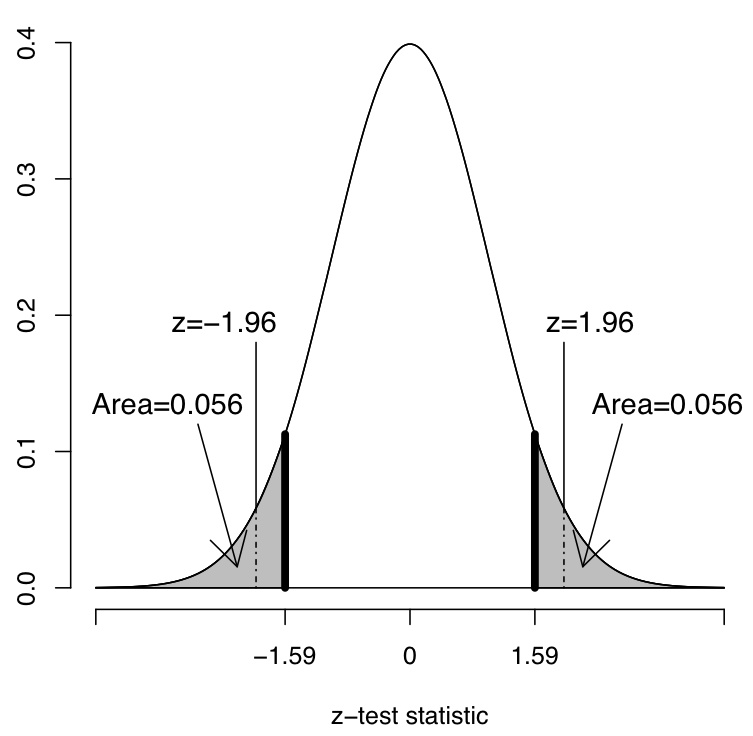
When the sample size is large enough, the sampling distribution of \(z\) defined by ((5.11)) is approximately the standard normal distribution. The probability curve of this distribution is shown in Figure 5.1. For now we just take it as given, and postpone a general discussion of the normal distribution until Chapter 7.
The \(P\)-value of the test is calculated from this distribution using the general principles introduced in Section 4.3.5. In other words, the \(P\)-value is the probability that the test statistic \(z\) has a value that is as or more extreme than the value of \(z\) in the observed sample. Now, however, the details of this calculation depend also on the alternative hypothesis, so some additional explanation is needed.
Consider first the more common case of a two-sided alternative hypothesis ((5.5)), that \(\Delta\ne 0\). As discussed in the previous section, it is large values of the test statistic which indicate evidence against the null hypothesis, because a large \(z\) is obtained when the sample difference \(\hat{\Delta}=\hat{\pi}-\pi_{0}\) is very different from the zero difference claimed by the null hypothesis. When the alternative is two-sided, “large” is taken to mean any value of \(z\) far from zero, i.e. either large positive or large negative values, because both indicate that the sample difference is far from 0. If \(z\) is large and positive, \(\hat{\Delta}\) is much larger than 0. In example 5.1 this would indicate that a much larger proportion than 0.5 of the sample say they intend to vote Yes. If \(z\) is large and negative, \(\hat{\Delta}\) is much smaller than 0, indicating a much smaller sample proportion than 0.5. Both of these cases would count as evidence against \(H_{0}\) when the alternative hypothesis is two-sided.
The observed value of the \(z\)-test statistic in Example 5.1 was actually \(z=-1.59\). Evidence would thus be “as strong” against \(H_{0}\) as the observed \(z\) if we obtained a \(z\)-test statistic of \(-1.59\) or 1.59, the value exactly as far from 0 as the observed \(z\) but above rather than below 0. Similarly, evidence against the null would be even stronger if \(z\) was further from zero than 1.59, i.e. larger than 1.59 or smaller than \(-1.59\). To obtain the \(P\)-value, we thus need to calculate the probability of observing a \(z\)-test statistic which is at most \(-1.59\) or at least 1.59 when the null hypothesis is true in the population. In general, the \(P\)-value for testing the null hypothesis against a two-sided alternative is the probability of obtaining a value at least \(z\) or at most \(-z\) (when \(z\) is positive, vice versa when it is negative), where \(z\) here denotes the value of the test statistic in the sample. Such probabilities are calculated from the approximately standard normal sampling distribution of the test statistic under \(H_{0}\).
This calculation of the \(P\)-value is illustrated graphically in Figure 5.1. The curve in the plot is that of the standard normal distribution. Two areas are shown in grey under the curve, one on each tail of the distribution. The one on the left corresponds to values of \(-1.59\) and smaller, and the one on the right to values of 1.59 or larger. Each of these areas is about 0.056, and the \(P\)-value for a test against a two-sided alternative is their combined area, i.e. \(P=0.056+0.056=0.112\). This means that even if the true population proportion of Yes-voters was actually exactly 0.5, there would be a probability of 0.112 of obtaining a test statistic as or more extreme than the \(z=-1.59\) that was actually observed in Example 5.1.
In example 5.2 the observed test statistic was \(z=-16.71\). The two-sided \(P\)-value is then the probability of values that are at most \(-16.71\) or at least 16.71. These areas are not shown in Figure 5.1 because they would not be visible in it. The horizontal axis of the figures runs from \(-4\) to \(+4\), so \(-16.71\) is clearly far in the tail of the distribution and the corresponding probability is very small; we would report it as \(P<0.001\).
Consider now the case of a one-sided alternative hypothesis. For example, in the referendum example we might have decided beforehand to focus only on the possiblity that the proportion of people who intend to vote Yes is smaller than 0.5, and hence consider the alternative hypothesis that \(\Delta<0\). Two situations might then arise. First, suppose that the observed value of the sample difference is in the direction indicated by the alternative hypothesis. This is the case in the example, where the sample difference \(\hat{\Delta}=-0.03\) is indeed smaller than zero, and the test statistic \(t=-1.59\) is negative. The possible values of \(z\) contributing to the \(P\)-value are then those of \(-1.59\) or smaller. Values of \(1.59\) and larger are now not included, because positive values of the test statistic (corresponding to sample differences greater than 0) would not be regarded as evidence in favour of the claim that \(\Delta\) is smaller than 0. The \(P\)-value is thus only the probability corresponding to the area on the left tail of the curve in Figure 5.1, and the corresponding area on the right tail is not included. Since both areas have the same size, the one-sided \(P\)-value is half the two-sided value, i.e. 0.056 instead of 0.112. In general, the one-sided \(P\)-value for a \(z\)-test of a proportion and other similar tests is always obtained by dividing the two-sided value by 2, if the sample evidence is in the direction of the one-sided alternative hypothesis.
The second case occurs when the sample difference is not in the direction indicated by a one-sided alternative hypothesis. For example, suppose that the sample proportion of Yes-voters had actually been 0.53, i.e. 0.03 larger than 0.5, so that we had obtained \(z=+1.59\) instead. The possible values of the test statistic which contributed to the \(P\)-value would then be \(z=1.59\) and all smaller values. These are “as strong or stronger evidence against the null hypothesis and in the direction of the alternative hypothesis” as required by the definition at the beginning of Section 4.3.5, since they agree with the alternative hypothesis (negative values of \(z\)) or at least disagree with it less than the observed \(z\) (positive values from 0 to 1.59). In Figure 5.1, these values would correspond to the area under the whole curve, apart from the region to the right of \(1.59\) on the right tail. Since the probability of the latter is 0.056 and the total probability under the curve is 1, the required probability is \(P=1-0.0.56=0.944\). However, calculating the \(P\)-value so precisely is hardly necessary in this case, as it is clearly going to be closer to 1 than to 0. The conclusion from such a large \(P\)-value will always be that the null hypothesis should not be rejected. This is also intuitively obvious, as a sample difference in the opposite direction from the one claimed by the alternative hypothesis is clearly not to be regarded as evidence in favour of that alternative hypothesis. In short, if the sample difference is in a different direction than a one-sided alternative hypothesis, the \(P\)-value can be reported simply as \(P>0.5\) without further calculations.
If a statistical software package is used to carry out the test, it will also report the \(P\)-value and no further calculations are needed (except dividing a two-sided \(P\)-value by 2, if a one-sided value is needed and only a two-sided one is reported). However, since SPSS does not currently provide a procedure for this test, and for exam purposes, we will briefly outline how an approximate \(P\)-value is obtained using critical values from a table. This is done in a very similar way as for the \(\chi^{2}\) test in Section 4.3.5.
The first part of Table 5.2 shows a table of critical values for the standard normal distribution. These values are also shown in the Appendix at the end of this course pack, on the last row of a larger table (the other parts of this table will be explained later, in Section 7.3.4). A version of this table is included in all introductory text books on statistics, although its format may be slightly different in different books.
| 0.100 | 0.050 | 0.025 | 0.01 | 0.005 | 0.001 | 0.0005 | |
| Critical value | 1.282 | 1.645 | 1.960 | 2.326 | 2.576 | 3.090 | 3.291 |
| Alternative hypothesis | Significance levels 0.10 | 0.05 | 0.01 | 0.001 |
| Two-sided | 1.65 | 1.96 | 2.58 | 3.29 |
| One-sided | 1.28 | 1.65 | 2.33 | 3.09 |
The columns of the first part of Table 5.2 are labelled “Right-hand tail probabilities”, with separate columns for some values from 0.100 to 0.0005. This means that the probability that a value from the standard normal distribution is at least as large as the value given in a particular column is the number given at the top of that column. For example, the value in the column labelled “0.025” is 1.960, indicating that the probability of obtaining a value equal to or greater than 1.960 from the standard normal distribution is 0.025. Because the distribution is symmetric, the probability of values of at most \(-1.960\) is also 0.025, and the total probability that a value is at least 1.960 units from zero is \(0.025+0.025=0.05\).
These values can be used to obtain bounds for \(P\)-values, expressed in terms of conventional significance levels of 0.10, 0.05, 0.01 and 0.001. The values at which these tail probabilities are obtained are the corresponding critical values for the test statistic. They are shown in the lower part of Table 5.2, slightly rearranged for clarity of presentation and rounded to two decimal places (which is accurate enough for practical purposes). The basic idea of using the critical values is that if the observed (absolute value of) the \(z\)-test statistic is larger than a critical value (for the required kind of alternative hypothesis) shown in the lower part of Table 5.2, the \(P\)-value is smaller than the significance level corresponding to that critical value.
The table shows only positive critical values. If the observed test statistic is actually negative, its negative (\(-\)) sign is omitted and the resulting positive value (i.e. the absolute value of the statistic) is compared to the critical values. Note also that the critical value for a given significance level depends on whether the alternative hypothesis is two-sided or one-sided. In the one-sided case, the test statistic is compared to the critical values only if it is actually in the direction of the alternative hypothesis; if not, we can simply report \(P>0.5\) as discussed above.
The \(P\)-value obtained from the table is reported as being smaller than the smallest conventional significance level for which the corresponding critical value is exceeded by the observed test statistic. For instance, in the jury example 5.2 we have \(z=-16.71\). Considering a two-sided alternative hypothesis, 16.71 is larger than the critical values 1.65, 1.96, 2.58 and 3.29 for all the standard significance levels, so we can report that \(P<0.001\). For Example 5.1, in contrast, \(z=-1.59\), the absolute value of which is smaller than even the critical value 1.65 for the 10% significance level. For this example, we would report \(P>0.1\).
The intuitive idea of the critical values and their connection to the \(P\)-values is illustrated for Example 5.1 by Figure 5.1. Here the observed test statistic is \(t=-1.59\), so the two-sided \(P\)-value is the probability of values at least 1.59 or at most \(-1.59\), which correspond to the two gray areas in the tails of the distribution. Also shown in the plot is one of the critical values for two-sided tests, the 1.96 for significance level 0.05. By definition of the critical values, the combined tail probability of values at least 1.96 from 0, i.e. the probability of values at least 1.96 or at most \(-1.96\), is 0.05. It is clear from the plot that since 1.59 is smaller than 1.96, these areas are smaller than the tail areas corresponding to 1.59 and \(-1.59\), and the combined area of the latter must be more than 0.05, i.e. it must be that \(P>0.05\). Similar argument for the 10% critical value of 1.65 shows that \(P\) is here also larger than 0.1.
5.5.4 Conclusions from the test
The general principles of drawing and stating conclusions from a significance test have already been explained in Section 4.3.6, so they need not be repeated here. Considering two-sided alternative hypotheses, the conclusions in our two examples are as follows:
In the referendum example 5.1, \(P=0.112\) for the null hypothesis that \(\pi=0.5\) in the population of eligible voters. The null hypothesis is not rejected at conventional levels of significance. There is not enough evidence to conclude that the proportion of voters who definitely intend to vote Yes differs from one half.
In the jury example 5.2, \(P<0.001\) for the null hypothesis that \(\pi=0.124\). The null hypothesis is thus overwhelmingly rejected at any conventional level of significance. There is very strong evidence that the probability of a black person being selected to the jury pool differs from the proportion of black people in the population of the county.
5.5.5 Summary of the test
As a summary, let us again repeat the main steps of the test described in this section in a concise form, using the voting variable of Example 5.1 for illustration:
Data: a sample of size \(n=702\) of a dichotomous variable \(Y\) with values 1 (Yes) and 0 (No or undecided), with the sample proportion of ones \(\hat{\pi}=0.47\).
Assumptions: the observations are a random sample from a population distribution with some population proportion (probability) \(\pi\), and the sample size \(n\) is large enough for the test to be valid (for example, \(n\ge 30\) when \(\pi_{0}\) is between about 0.3 and 0.7, as it is here).
Hypotheses: null hypothesis \(H_{0}: \pi=\pi_{0}\) against the alternative hypothesis \(H_{a}: \pi\ne \pi_{0}\), where \(\pi_{0}=0.5\).
The test statistic: the \(z\)-statistic \[z=\frac{\hat{\pi}-\pi_{0}}{\sqrt{\pi_{0}(1-\pi_{0})/n}}= \frac{0.47-0.50}{\sqrt{0.50\times(1-0.50)/702}}=-1.59.\]
The sampling distribution of the test statistic when \(H_{0}\) is true: a standard normal distribution.
-
The \(P\)-value: the probability that a randomly selected value from the the standard normal distribution is at most \(-1.59\) or at least 1.59, which is \(P=0.112\).
- If the precise \(P\)-value is not available, we can observe that 1.59 is smaller than the two-sided critical value 1.65 for the 10% level of significance. Thus it must be that \(P>0.1\).
Conclusion: The null hypothesis is not rejected (\(P=0.112\)). There is not enough evidence to conclude that the proportion of eligible voters who definitely intend to vote Yes differs from one half. Based on this opinion poll, the referendum remains too close to call.
5.6 Confidence interval for a single proportion
5.6.1 Introduction
A significance test assesses whether it is plausible, given the evidence in the observed data, that a population parameter or parameters have a specific set of values claimed by the null hypothesis. For example, in Section 5.5 we asked such a question about the probability parameter of a binary variable in a single population.
In many ways a more natural approach would be try to identify all of those values of a parameter which are plausible given the data. This leads to a form of statistical inference known as interval estimation, which aims to present not only a single best guess (i.e. a point estimate) of a population parameter, but also a range of plausible values (an interval estimate) for it. Such an interval is known as a confidence interval. This section introduces the idea of confidence intervals, and shows how to construct them for a population probability. In later sections, the same principles will be used to calculate confidence intervals for other kinds of population parameters.
Interval estimation is an often underused part of statistical inference, while significance testing is arguably overused or at least often misused. In most contexts it would be useful to report confidence intervals in addition to, or instead of, results of significance tests. This is not done often enough in research publications in the social sciences.
5.6.2 Calculation of the interval
Our aim is again to draw inference on the difference \(\Delta=\pi-\pi_{0}\) or, equivalently, the population probability \(\pi\). The point estimate of \(\Delta\) is \(\hat{\Delta}=\hat{\pi}-\pi_{0}\) where \(\hat{\pi}\) is the sample proportion corresponding to \(\pi\). Suppose that the conditions on the sample size \(n\) that were discussed in Section 5.5.3 are again satisfied.
Consider now Figure @ref(fig:f-pval-prob}. One of the results illustrated by it is that if \(\pi_{0}\) is the true value of of the population probability \(\pi\), so that \(\Delta=\pi-\pi_{0}=0\), there is a probability of 0.95 that for a randomly drawn sample from the population the \(z\)-test statistic \(z=\hat{\Delta}/\hat{\sigma}_{\hat{\Delta}}\) is between \(-1.96\) and \(+1.96\). This also implies that the probability is 0.95 that in such a sample the observed value of \(\hat{\Delta}\) will be between \(\Delta-1.96\,\hat{\sigma}_{\hat{\Delta}}\) and \(\Delta+1.96\,\hat{\sigma}_{\hat{\Delta}}\). Furthermore, it is clear from the figure that all of the values within this interval are more likely to occur than any of the values outside the interval (i.e. those in the two tails of the sampling distribution). The interval thus seems like a sensible summary of the “most likely” values that the estimate \(\hat{\Delta}\) may have in random samples.
A confidence interval essentially turns this around, into a statement about the unknown true value of \(\Delta\) in the population, even in cases where \(\Delta\) is not 0. This is done by substituting \(\hat{\Delta}\) for \(\Delta\) above, to create the interval \[\begin{equation} \text{from }\hat{\Delta} -1.96\times \hat{\sigma}_{\hat{\Delta}}\text{ to }\hat{\Delta}+1.96\times \hat{\sigma}_{\hat{\Delta}}. \tag{5.12} \end{equation}\] This is the 95 % confidence interval for the population difference \(\Delta\). It is usually written more concisely as \[\begin{equation} \hat{\Delta}\pm 1.96\, \hat{\sigma}_{\hat{\Delta}} \tag{5.13} \end{equation}\] where the “plusminus” symbol \(\pm\) indicates that we calculate the two endpoints of the interval as in ((5.12)), one below and one above \(\hat{\Delta}\).
Expression ((5.13)) is general in the sense that many different quantities can take the role of \(\Delta\) in it. Here we consider for now the case of \(\Delta=\pi-\pi_{0}\). The estimated standard error \(\hat{\sigma}_{\hat{\Delta}}\) is analogous to ((5.10)) used for the \(z\)-test, but not the same. This is because the confidence interval is not calculated under the null hypothesis \(H_{0}:\; \pi=\pi_{0}\), so we cannot use \(\pi_{0}\) for \(\pi\) in the standard error. Instead, \(\pi\) is estimated by the sample proportion \(\hat{\pi}\), giving the estimated standard error[^] \[\begin{equation} \hat{\sigma}_{\hat{\Delta}} = \sqrt{\frac{\hat{\pi}(1-\hat{\pi})}{n}} \tag{5.14} \end{equation}\] and thus the 95% confidence interval \[(\hat{\pi}-\pi_{0}) \pm 1.96 \; \sqrt{ \frac{\hat{\pi}(1-\hat{\pi})}{n}}\] for \(\Delta=\pi-\pi_{0}\). Alternatively, a confidence interval for \(\pi\) itself is given by \[\begin{equation} \hat{\pi} \pm 1.96 \;\sqrt{\frac{\hat{\pi}(1-\hat{\pi})}{n}}. \tag{5.15} \end{equation}\] This is typically the most useful interval for use in practice. For instance, in the referendum example 5.1 this gives a 95% confidence interval of \[0.470\pm 1.96\times \sqrt{\frac{0.470\times(1-0.470)}{702}} =0.470\pm 0.0369=(0.433, 0.507)\] for the proportion of definite Yes-voters in the population. Similarly, in Example 5.2 the 95% confidence interval for the probability of a black person being selected for the jury pool is (0.040, 0.052). These intervals are also shown in Table 5.1.
5.6.3 Interpretation of confidence intervals
As with the \(P\)-value of a significance test, the precise interpretation of a confidence interval refers to probabilities calculated from a sampling distribution, i.e. probabilities evaluated from a hypothetical exercise of repeated sampling:
- If we obtained many samples from the population and calculated the confidence interval for each such sample using the formula ((5.15)), approximately 95% of these intervals would contain the true value of the population proportion \(\pi\).
This is undeniably convoluted, even more so than the precise interpretation of a \(P\)-value. In practise a confidence interval would not usually be described in exactly these words. Instead, a research report might, for example, write that (in the referendum example) “the 95 % confidence interval for the proportion of eligible voters in the population who definitely intend to vote Yes is (0.433, 0.507)”, or that “we are 95 % confident that the proportion of eligible voters in the population who definitely intend to vote Yes is between 43.3% and 50.7%”. Such a statement in effect assumes that the readers will be familiar enough with the idea of confidence intervals to understand the claim. It is nevertheless useful to be aware of the more careful interpretation of a confidence interval, if only to avoid misunderstandings. The most common error is to claim that “there is a 95% probability that the proportion in the population is between 0.433 and 0.507”. Although the difference to the interpretation given above may seem small, the latter statement is not really true, or strictly speaking even meaningful, in the statistical framework considered here.
In place of the 1.96 in ((5.13)), we may also use other numbers. To allow for this in the notation, we can also write \[\begin{equation} \hat{\Delta} \pm z_{\alpha/2}\; \hat{\sigma}_{\hat{\Delta}}. \tag{5.16} \end{equation}\] where the multiplier \(z_{\alpha/2}\) is a number which depends on two things. One of them is the sampling distribution of \(\hat{\Delta}\), which is here assumed to be the normal distribution (another possibility is discussed in Section 7.3.4). The second is the confidence level which we have chosen for the confidence interval. For example, the probability of 0.95 in the interpretation of a 95% confidence interval discussed above is the confidence level of that interval. Conventionally the 0.95 level is most commonly used, while other standard choices are 0.90 and 0.99, i.e. 90% and 99% confidence intervals.
In the symbol \(z_{\alpha/2}\), \(\alpha\) is a number such that \(1-\alpha\) equals the required confidence level. In other words, \(\alpha=0.1\), 0.05, and 0.01 for confidence levels of \(1-\alpha=0.90\), 0.95 and 0.99 respectively. The values that are required for the conventional levels are \(z_{0.10/2}=z_{0.05}=1.64\), \(z_{0.05/2}=z_{0.025}=1.96\), and \(z_{0.01/2}=z_{0.005}=2.58\), which correspond to intervals at the confidence levels of 90%, 95% and 99% respectively. These values are also shown in Table 5.3.
| Confidence levels: | |||
| 90% | 95% | 99% | |
| Multiplier \(z_{\alpha/2}\) | 1.64 | 1.96 | 2.58 |
A confidence interval contains, loosely speaking, those numbers which are considered plausible values for the unknown population difference \(\Delta\) in the light of the evidence in the data. The width of the interval thus reflects our uncertainty about the exact value of \(\Delta\), which in turn is related to the amount of information the data provide about \(\Delta\). If the interval is wide, many values are consistent with the observed data, so there is still a large amount of uncertainty; if the interval is narrow, we have much information about \(\Delta\) and thus little uncertainty. Another way of stating this is that when the confidence interval is narrow, estimates of \(\Delta\) are very precise.
The width of the interval ((5.16)) is \(2\times z_{\alpha/2}\times \hat{\sigma}_{\hat{\Delta}}\). This depends on
The confidence level: the higher the level, the wider the interval. Thus a 99% confidence interval is always wider than a 95% interval for the same data, and wider still than a 90% interval. This is logically inevitable: if we want to state with high level of confidence that a parameter is within a certain interval, we must allow the interval to contain a wide range of values. It also explains why we do not consider a 100% confidence interval: this would contain all possible values of \(\Delta\) and exclude none, making no use of the data at all. Instead, we aim for a high but not perfect level of confidence, obtaining an interval which contains some but not all possible values, for the price of a small chance of incorrect conclusions.
-
The standard error \(\hat{\sigma}_{\hat{\Delta}}\), which in the case of a single proportion is ((5.14)). This in turn depends on
the sample size \(n\): the larger this is, the narrower the interval. Increasing the sample size thus results (other things being equal) in reduced uncertainty and higher precision.
the true population proportion \(\pi\): the closer this is to 0.5, the wider the interval. Unlike the sample size, this determinant of the estimation uncertainty is not in our control.
Opinion polls of the kind illustrated by the referendum example are probably where non-academic audiences are most likely to encounter confidence intervals, although not under that label. Media reports of such polls typically include a margin of error for the results. For example, in the referendum example it might be reported that 47% of the respondents said that they would definitely vote Yes, and that “the study has a margin of error of plus or minus four percentage points”. In most cases the phrase “margin of error” refers to a 95% confidence interval. Unless otherwise mentioned, we can thus take a statement like the one above to mean that the 95% confidence interval for the proportion of interest is approximately \(47\pm 4\) percentage points. For a realistic interpretation of the implications of the results, the width of this interval is at least as important as the point estimate of the proportion. This is often neglected in media reports of opinion polls, where the point estimate tends to be headline news, while the margin of error is typically mentioned only in passing or omitted altogether.
5.6.4 Confidence intervals vs. significance tests
There are some obvious similarities between the conclusions from significance tests and confidence intervals. For example, a \(z\)-test in the referendum example 5.1 showed that the null hypothesis that the population proportion \(\pi\) was 0.5 was not rejected (\(P=0.112\)). Thus 0.5 is a plausible value for \(\pi\) in light of the observed data. The 95% confidence interval for \(\pi\) showed that, at this level of confidence, plausible values for \(\pi\) are those between 0.433 and 0.507. In particular, these include 0.5, so the confidence interval also indicates that a proportion of 0.5 is plausible. This connection between the test and the confidence interval is in fact exact:
- If the hypothesis \(H_{0}: \Delta=0\) about a population quantity \(\Delta\) is rejected at the 5% level of significance using the \(z\)-test against a two-sided alternative hypothesis, the 95 % confidence interval for \(\Delta\) will not contain 0, and vice versa. Similarly, if \(H_{0}\) is not rejected, the confidence interval will contain 0, and vice versa.
The same is true for other matching pairs of levels of significance and confidence, e.g. for a test with a 1% level of significance and a 99% (i.e. (100-1)%) confidence interval. In short, the significance test and the confidence interval will in these cases always give the same answer about whether or not a parameter value is plausible (consistent with the data) at a given level of significance/confidence.
These pairs of a test and an interval are exactly comparable in that they concern the same population parameter, estimate all parameters in the same way, use the same sampling distribution for inference, and use the same level of significance/confidence. Not all tests and confidence intervals have exact pairs in this way. Also, some tests are for hypotheses about more than one parameter at once, so there is no corresponding single confidence interval. Nevertheless, the connection stated above is useful for understanding the ideas of both tests and confidence intervals.
These results also illustrate how confidence intervals are inherently more informative than significance tests. For instance, in the jury example 5.2, both the test and the confidence interval agree on the implausibility of the claim that the population probability of being selected to the jury panel is the same as the proportion (0.124) of black people in the population, since the claim that \(\pi=0.124\) is rejected by the test (with \(P<0.001\)) and outside the interval \((0.040; 0.052)\). Unlike the test, however, the confidence interval summarizes the plausibility of all possible values of \(\pi\) and not just \(\pi_{0}=0.124\). One way to describe this is to consider what would have happened if we had carried out a series of significance tests of null hypotheses of the form \(H_{0}: \pi=\pi_{0}\) for a range of values of \(\pi_{0}\). The confidence interval contains all those values \(\pi_{0}\) which would not have been rejected by the test, while all the values outside the interval would have been rejected. Here \(H_{0}: \pi=\pi_{0}\) would thus not have been rejected at the 5% level if \(\pi_{0}\) had been between 0.040 and 0.052, and rejected otherwise. This, of course, is not how significance tests are actually conducted, but it provides a useful additional interpretation of confidence intervals.
A confidence interval is particularly useful when the parameter of interest is measured in familiar units, such as the proportions considered so far. We may then try to judge, in substantive terms, how wide the interval is and how far it is from particular values of interest. In the jury example the 95% confidence interval ranges from 4.0% to 5.2%, which suggests that the population probability is estimated fairly precisely by this survey. The interval also reveals that even its upper bound is less than half of the figure of 12.4% which would correspond to proportional representation of black people in the jury pool, a result which suggests quite substantial underrepresentation in the pool.
5.7 Inference for comparing two proportions
In Examples 5.3 and 5.4, the aim is to compare the proportion of a dichotomous response variable \(Y\) between two groups of a dichotomous explanatory variable \(X\):
Example 5.3: compare the proportion of polio cases among the unvaccinated (\(\pi_{1}\)) and vaccinated (\(\pi_{2}\)) children.
Example 5.4: compare the proportion of optimistic responses to a negative (\(\pi_{1}\)) vs. positive wording of the question (\(\pi_{2}\)).
The quantity of interest is then the population difference \[\begin{equation} \Delta=\pi_{2}-\pi_{1}. \tag{5.17} \end{equation}\] For a significance test of this, the null hypothesis will again be \(H_{0}:\; \Delta=0\), which is in this case equivalent to the hypothesis of equal proportions \[\begin{equation} H_{0}:\; \pi_{1} = \pi_{2}. \tag{5.18} \end{equation}\] The null hypothesis thus claims that there is no association between the group variable \(X\) and the dichotomous response variable \(Y\), while the alternative hypothesis (e.g. the two-sided one \(H_{a}:\; \pi_{1}\ne \pi_{2}\), i.e. \(H_{a}:\; \Delta\ne 0\)) implies that there is an association.
The obvious estimates of \(\pi_{1}\) and \(\pi_{2}\) are the corresponding sample proportions \(\hat{\pi}_{1}\) and \(\hat{\pi}_{2}\), calculated from samples of sizes \(n_{1}\) and \(n_{2}\) respectively, and the estimate of \(\Delta\) is then \[\begin{equation} \hat{\Delta}=\hat{\pi}_{2} - \hat{\pi}_{1}. \tag{5.19} \end{equation}\] This gives \(\hat{\Delta}=0.000284-0.000706=-0.000422\) in Example 5.3 and \(\hat{\Delta}=0.364-0.279=0.085\) in Example 5.4. In the samples, the proportion of polio cases is thus lower in the vaccinated group, and the proportion of optimistic answers is higher in response to a positively worded question. Note also that although the inference discussed below focuses on the difference of the proportions, for purely descriptive purposes we might prefer to use some other statistic, such as the ratio of the proportions. For example, the difference of 0.000422 in polio incidence between vaccine and control groups may seem small, because the proportions in both groups are small. A better idea of the the magnitude of the contrast is given by their ratio of \(0.000706/0.000284=2.49\) (this is known as the risk ratio). In other words, the rate of polio infection in the unvaccinated group was two and a half times the rate in the vaccinated group.
The tests and confidence intervals discussed below are again based on the assumption that the relevant sampling distributions are approximately normal, which is true when the sample sizes \(n_{1}\) and \(n_{2}\) are large enough. The conditions for this are not very demanding: one rule of thumb states that the methods described in this section are reasonably valid if in both groups the number of observations with \(Y\) having the value 1, and of ones with the value 0, are both more than 5. This condition is satisfied in both of the examples considered here.
The validity of the test, as well as the amount of information the data provide about \(\pi_{1}\) and \(\pi_{2}\) in general, thus depends not just on the overall sample sizes but on having enough observations of both values of \(Y\). The critical quantity is then the number of observations in the rarer category of \(Y\). In Example 5.3 this means the numbers of children diagnosed with polio, because the probability of polio was low in the study population. The numbers of eventual polio cases were 142 and 57 in the control and treatment groups respectively, so the rule of thumb stated above was satisfied. With such low probabilities of polio incidence, sufficient numbers of cases were achieved only by making the overall sample sizes \(n_{1}\) and \(n_{2}\) large enough. That is why the trial had to be very large, involving hundreds of thousands of participants.
The standard error of \(\hat{\Delta}\) is \[\begin{equation} \sigma_{\hat{\Delta}} =\sqrt{\frac{\pi_{2}(1-\pi_{2})}{n_{2}}+\frac{\pi_{1}(1-\pi_{1})}{n_{1}}}. \tag{5.20} \end{equation}\] As in the one-sample case above, the best way to estimate this is different for a significance test than for a confidence interval. For a test, the standard error can be estimated under assumption that the null hypothesis ((5.18)) is true, in which case the population proportion is the same in both groups. A good estimate of this common proportion, denoted below by \(\hat{\pi}\), is the proportion of observations with value 1 for \(Y\) in the total sample of \(n_{1}+n_{2}\) observations, pooling observations from both groups together; expressed in terms of the group-specific estimates, this is \[\begin{equation} \hat{\pi} = \frac{n_{1}\hat{\pi}_{1}+n_{2}\hat{\pi}_{2}}{n_{1}+n_{2}}. \tag{5.21} \end{equation}\] Using this for both \(\pi_{1}\) and \(\pi_{2}\) in ((5.20)) gives the estimated standard error \[\begin{equation} \hat{\sigma}_{\hat{\Delta}}=\sqrt{\hat{\pi}(1-\hat{\pi}) \; \left(\frac{1}{n_{2}}+\frac{1}{n_{1}}\right),} \tag{5.22} \end{equation}\] and using ((5.19)) and ((5.22)) in the general formula ((5.8)) gives the two-sample \(z\)-test statistic for proportions \[\begin{equation} z=\frac{\hat{\pi}_{2}-\hat{\pi}_{1}}{\sqrt{\hat{\pi}(1-\hat{\pi})(1/n_{2}+1/n_{1})}} \tag{5.23} \end{equation}\] where \(\hat{\pi}\) is given by ((5.21)). When the null hypothesis is true, the sampling distribution of this test statistic is approximately standard normal when the sample sizes are large enough.
For a confidence interval, the calculation of the estimated standard error cannot assume that ((5.18)) is true. Instead, we use the estimate \[\begin{equation} \hat{\sigma}_{\hat{\Delta}} =\sqrt{\frac{\hat{\pi}_{2}(1-\hat{\pi}_{2})}{n_{2}}\frac{\hat{\pi}_{1}(1-\hat{\pi}_{1})}{n_{1}}} \tag{5.24} \end{equation}\] and, substituting this to the general formula ((5.16)), we get \[\begin{equation} (\hat{\pi}_{2}-\hat{\pi}_{1}) \pm z_{\alpha/2} \;\sqrt{\frac{\hat{\pi}_{2}(1-\hat{\pi}_{2})}{n_{2}} +\frac{\hat{\pi}_{1}(1-\hat{\pi}_{1})}{n_{1}}} \tag{5.25} \end{equation}\] as the confidence interval for \(\Delta=\pi_{2}-\pi_{1}\), with confidence level \(1-\alpha\).
For an illustration of the calculations, consider Example 5.4. Denoting the group of respondents answering the negatively worded question by 1 and those with the positive question by 2, the basic quantities are \(n_{1}=921\), \(\hat{\pi}_{1}=0.279\), \(n_{2}=929\) and \(\hat{\pi}_{2}=0.364\). The estimated difference in the proportions of respondents giving an optimistic answer is thus \[\hat{\Delta} = \hat{\pi}_{2}-\hat{\pi}_{1} = 0.364-0.279 = 0.085.\] For a significance test, the estimated standard error of \(\hat{\Delta}\) uses the pooled estimate ((5.21)) of the population proportion, which is given by \[\hat{\pi} = \frac{921\times 0.279+929\times 0.364}{921+929}= \frac{257+338}{921+929} = 0.322.\] The standard error from ((5.22)) is then \[\hat{\sigma}_{\hat{\Delta}} = \sqrt{ 0.322\times(1-0.322) \times \left( \frac{1}{929}+ \frac{1}{921} \right) } = \sqrt{ \frac{0.2182}{462.5} }=0.0217,\] and the test statistic ((5.23)) is \[z=\frac{0.085}{0.0217}=3.92.\] For the confidence interval, the standard error of \(\hat{\Delta}\) is estimated from ((5.24)) as \[\begin{aligned} \hat{\sigma}_{\hat{\Delta}} &=& \sqrt{ \frac{0.364\times (1-0.364)}{929} + \frac{0.279\times (1-0.279)}{921} } \\ &=& \sqrt{ \frac{0.2315}{929} +\frac{0.2012}{921} }=0.0216\end{aligned}\] and a 95% confidence interval from ((5.25)) is \[0.085 \pm 1.96 \times 0.0216 = 0.085\pm 0.042 = (0.043; 0.127).\] The \(P\)-value for the test statistic is clearly very low (in fact about \(0.00009\)), so the null hypothesis of equal proportions is convincingly rejected. There is very strong evidence that the probability that a respondent will give an answer indicating optimism for the future is different for the two differently worded questions. The confidence interval indicates that we are 95% confident that the proportion of optimistic answers is between 4.3 and 12.7 percentage points higher when the question is worded positively than when it is worded negatively. This suggests quite a substantial acquiescence bias arising from changing just one word in the survey question, as described in the introduction to Example 5.4 at the beginning of this chapter.
In Example 5.3, the estimated difference is \(\hat{\Delta}=-0.000422\) (see Table 5.1, i.e. 422 fewer polio cases per million children in the vaccinated group than in the unvaccinated group. Similar calculations as above show that the value of the test statistic is \(z=-6.01\), so the \(P\)-value is again very small (in fact about 0.000000001) and the null hypothesis of equal probabilities is strongly rejected. There is thus overwhelming evidence that the proportion of polio cases was different among the vaccinated children than among the unvaccinated ones. The 95% confidence interval for the difference shows that we are 95% confident that this difference was a reduction of between 284 and 560 polio cases per million children.23 This was acknowledged as a convincing demonstration that the Salk vaccine worked (see Figure 5.2), and it (and later other types of polio vaccination) was soon put to widespread use. The resulting dramatic decline in the incidence of polio is one of the great success stories of modern medicine. Compared to the 199 children with polio in 1954 among the less than half a million participants of the vaccine trial alone, in 2014 there were 414 confirmed cases of polio in the whole world (see http://www.polioeradication.org/Dataandmonitoring/Poliothisweek.aspx). There is hope that that number will reach 0 in a not-too-distant future, so that the once devastating disease will one day be entirely eradicated.