Chapter 7 Analysis of population means

7.1 Introduction and examples

This chapter introduces some basic methods of analysis for continuous, interval-level variables. The main focus is on statistical inference on population means of such variables, but some new methods of descriptive statistics are also described. The discussion draws on the general ideas that have already been explaned for inference in Chapters 4 and 5, and for continuous distributions in Chapter 6. Few if any new concepts thus need to be introduced here. Instead, this chapter can focus on describing the specifics of these very commonly used methods for continuous variables.

As in Chapter 5, questions on both a single group and on comparisons between two groups are discussed here. Now, however, the main focus is on the two-group case. There we treat the group as the explanatory variable \(X\) and the continuous variable of interest as the response variable \(Y\), and assess the possible associations between \(X\) and \(Y\) by comparing the distributions (and especially the means) of \(Y\) in the two groups.

The following five examples will be used for illustration throughout this chapter. Summary statistics for them are shown in Table 7.1.

Example 7.1: Survey data on diet

The National Diet and Nutrition Survey of adults aged 19–64 living in private households in Great Britain was carried out in 2000–01.²⁸ One part of the survey was a food diary where the respondents recorded all food and drink they consumed in a seven-day period. We consider two variables derived from the diary: the consumption of fruit and vegetables in portions (of 400g) per day (with mean in the sample of size \(n=1724\) of \(\bar{Y}=2.8\), and standard deviation \(s=2.15\)), and the percentage of daily food energy intake obtained from fat and fatty acids (\(n=1724\), \(\bar{Y}=35.3\), and \(s=6.11\)).

One sample	\(n\)	\(\bar{Y}\)	\(s\)	Diff.
Example 7.1: Variables from the National Diet and Nutrition Survey
Fruit and vegetable consumption (400g portions)	1724	2.8	2.15
Total energy intake from fat (%)	1724	35.3	6.11
Two independent samples
Example 7.2: Average weekly hours spent on housework
Men	635	7.33	5.53
Women	469	8.49	6.14	1.16
Example 7.3: Perceived friendliness of a police officer
No sunglasses	67	8.23	2.39
Sunglasses	66	6.49	2.01	-1.74
Two dependent samples
Example 7.4: Father’s personal well-being
Sixth month of wife’s pregnancy	109	30.69
One month after the birth	109	30.77	2.58	0.08
Example 7.5: Traffic flows on successive Fridays
Friday the 6th	10	128,385
Friday the 13th	10	126,550	1176	-1835

:(#tab:t-groupex)Examples of analyses of population means used in Chapter 7. Here \(n\) and \(\bar{Y}\) denote the sample size and sample mean respectively, in the two-group examples 7.2–7.5 separately for the two groups. “Diff.” denotes the between-group difference of means, and \(s\) is the sample standard deviation of the response variable \(Y\) for the whole sample (Example 7.1), of the response variable within each group (Examples 7.2 and 7.3), or of the within-pair differences (Examples 7.4 and 7.5).

Example 7.2: Housework by men and women

This example uses data from the 12th wave of the British Household Panel Survey (BHPS), collected in 2002. BHPS is an ongoing survey of UK households, measuring a range of socioeconomic variables. One of the questions in 2002 was

“About how many hours do you spend on housework in an average week, such as time spent cooking, cleaning and doing the laundry?”

The response to this question (recorded in whole hours) will be the response variable \(Y\), and the respondent’s sex will be the explanatory variable \(X\). We consider only those respondents who were less than 65 years old at the time of the interview and who lived in single-person households (thus the comparisons considered here will not involve questions of the division of domestic work within families).²⁹

We can indicate summary statistics separately for the two groups by using subscripts 1 for men and 2 for women (for example). The sample sizes are \(n_{1}=635\) for men and \(n_{2}=469\) for women, and the sample means of \(Y\) are \(\bar{Y}_{1}=7.33\) and \(\bar{Y}_{2}=8.49\). These and the sample standard deviations \(s_{1}\) and \(s_{2}\) are also shown in Table 7.1.

Example 7.3: Eye contact and perceived friendliness of police officers

This example is based on an experiment conducted to examine the effects of some aspects of the appearance and behaviour of police officers on how members of the public perceive their encounters with the police.³⁰ The subjects of the study were 133 people stopped by the Traffic Patrol Division of a detachment of the Royal Canadian Mounted Police. When talking to the driver who had been stopped, the police officer either wore reflective sunglasses which hid his eyes, or wore no glasses at all, thus permitting eye contact with the respondent. These two conditions define the explanatory variable \(X\), coded 1 if the officer wore no glasses and 2 if he wore sunglasses. The choice of whether sunglasses were worn was made at random before a driver was stopped.

While the police officer went back to his car to write out a report, a researcher asked the respondent some further questions, one of which is used here as the response variable \(Y\). It is a measure of the respondent’s perception of the friendliness of the police officer, measured on a 10-point scale where large values indicate high levels of friendliness.

The article describing the experiment does not report all the summary statistics needed for our purposes. The statistics shown in Table 7.1 have thus been partially made up for use here. They are, however, consistent with the real results from the study. In particular, the direction and statistical significance of the difference between \(\bar{Y}_{2}\) and \(\bar{Y}_{1}\) are the same as those in the published report.

Example 7.4: Transition to parenthood

In a study of the stresses and feelings associated with parenthood, 109 couples expecting their first child were interviewed before and after the birth of the baby.³¹ Here we consider only data for the fathers, and only one of the variables measured in the study. This variable is a measure of personal well-being, obtained from a seven-item attitude scale, where larger values indicate higher levels of well-being. Measurements of it were obtained for each father at three time points: when the mother was six months pregnant, one month after the birth of the baby, and six months after the birth. Here we will use only the first two of the measurements. The response variable \(Y\) will thus be the measure of personal well-being, and the explanatory variable \(X\) will be the time of measurement (sixth month of the pregnancy or one month after the birth). The means of \(Y\) at the two times are shown in Table 7.1. As in Example 7.3, not all of the numbers needed here were given in the original article. Specifically, the standard error of the difference in Table 7.1 has been made up in such a way that the results of a significance test for the mean difference agree with those in the article.

Example 7.5: Traffic patterns on Friday the 13th

A common superstition regards the 13th day of any month falling on a Friday as a particularly unlucky day. In a study examining the possible effects of this belief on people’s behaviour,³² data were obtained on the numbers of vehicles travelling between junctions 7 and 8 and junctions 9 and 10 on the M25 motorway around London during every Friday the 13th in 1990–92. For comparison, the same numbers were also recorded during the previous Friday (i.e. the 6th) in each case. There are only ten such pairs here, and the full data set is shown in Table 7.2. Here the explanatory variable \(X\) indicates whether a day is Friday the 6th (coded as 1) or Friday the 13th (coded as 2), and the response variable is the number of vehicles travelling between two junctions.

Date	Junctions	Friday the 6th	Friday the 13th	Difference
July 1990	7 to 8	139246	138548	-698
July 1990	9 to 10	134012	132908	-1104
September 1991	7 to 8	137055	136018	-1037
September 1991	9 to 10	133732	131843	-1889
December 1991	7 to 8	123552	121641	-1911
December 1991	9 to 10	121139	118723	-2416
March 1992	7 to 8	128293	125532	-2761
March 1992	9 to 10	124631	120249	-4382
November 1992	7 to 8	124609	122770	-1839
November 1992	9 to 10	117584	117263	-321

:(#tab:t-F13)Data for Example 7.5: Traffic flows between junctions of the M25 on each Friday the 6th and Friday the 13th in 1990-92.

In each of these cases, we will regard the variable of interest \(Y\) as a continuous, interval-level variable. The five examples illustrate three different situations considered in this chapter. Example 7.1 includes two separate \(Y\)-variables (consumption of fruit and vegetables, and fat intake), each of which is considered for a single population. Questions of interest are about the mean of the variable in the population. This is analogous to the one-group questions on proportions in Sections 5.5 and 5.6. In this chapter the one-group case is discussed only relatively briefly, in Section 7.4.

The main focus here is on the case illustrated by Examples 7.2 and 7.3. These involve samples of a response variable (hours of housework, or preceived friendliness) from two groups (men and women, or police with or without sunglasses). We are then interested in comparing the distributions, and especially the means, of the response variable between the groups. This case will be discussed first. Descriptive statistics for it are described in Section 7.2, and statistical inference in Section 7.3.

Finally, examples 7.4 and 7.5 also involve comparisons between two groups, but of a slightly different kind than examples 7.2 and 7.3. The two types of cases differ in the nature of the two samples (groups) being compared. In Examples 7.2 and 7.3, the samples can be considered to be independent. What this claim means will be discussed briefly later; informally, it is justified in these examples because the subjects in the two groups are separate and unrelated individuals. In Examples 7.4 and 7.5, in contrast, the samples (before and after the birth of a child, or two successive Fridays) must be considered dependent, essentially because they concern measurements on the same units at two distinct times. This case is discussed in Section 7.5.

In each of the four two-group examples we are primarily interested in questions about possible association between the group variable \(X\) and the response variable \(Y\). As before, this is the question of whether the conditional distributions of \(Y\) are different at the two levels of \(X\). There is thus an association between \(X\) and \(Y\) if

• Example 7.2: The distribution of hours of housework is different for men than for women.

• Example 7.3: The distribution of perceptions of a police officer’s friendliness is different when he is wearing mirrored sunglasses than when he is not.

• Example 7.4: The distribution of measurements of personal well-being is different at the sixth month of the pregnancy than one month after the birth.

• Example 7.5: The distributions of the numbers of cars on the motorway differ between Friday the 6th and the following Friday the 13th.

We denote the two values of \(X\), i.e. the two groups, by 1 and 2. The mean of the population distribution of \(Y\) given \(X=1\) will be denoted \(\mu_{1}\) and the standard deviation \(\sigma_{1}\), and the mean and standard deviation of the population distribution given \(X=2\) are denoted \(\mu_{2}\) and \(\sigma_{2}\) similarly. The corresponding sample quantities are the conditional sample means \(\bar{Y}_{1}\) and \(\bar{Y}_{2}\) and sample standard deviations \(s_{1}\) and \(s_{2}\). For inference, we will focus on the population difference \(\Delta=\mu_{2}-\mu_{1}\) which is estimated by the sample difference \(\hat{\Delta}=\bar{Y}_{2}-\bar{Y}_{1}\). Some of the descriptive methods described in Section 7.2, on the other hand, also aim to summarise and compare other aspects of the two conditional sample distributions.

7.2 Descriptive statistics for comparisons of groups

7.2.1 Graphical methods of comparing sample distributions

There is an association between the group variable \(X\) and the response variable \(Y\) if the distributions of \(Y\) in the two groups are not the same. To determine the extent and nature of any such association, we need to compare the two distributions. This section describes methods of doing so for observed data, i.e. for examining associations in a sample. We begin with graphical methods which can be used to detect differences in any aspects of the two distributions. We then discuss some non-graphical summaries which compare specific aspects of the sample distributions, especially their means.

Although the methods of inference described later in this chapter will be limited to the case where the group variable \(X\) is dichotomous, many of the descriptive methods discussed below can just as easily be applied when more than two groups are being compared. This will be mentioned wherever appropriate. For inference in the multiple-group case some of the methods discussed in Chapter 8 are applicable.

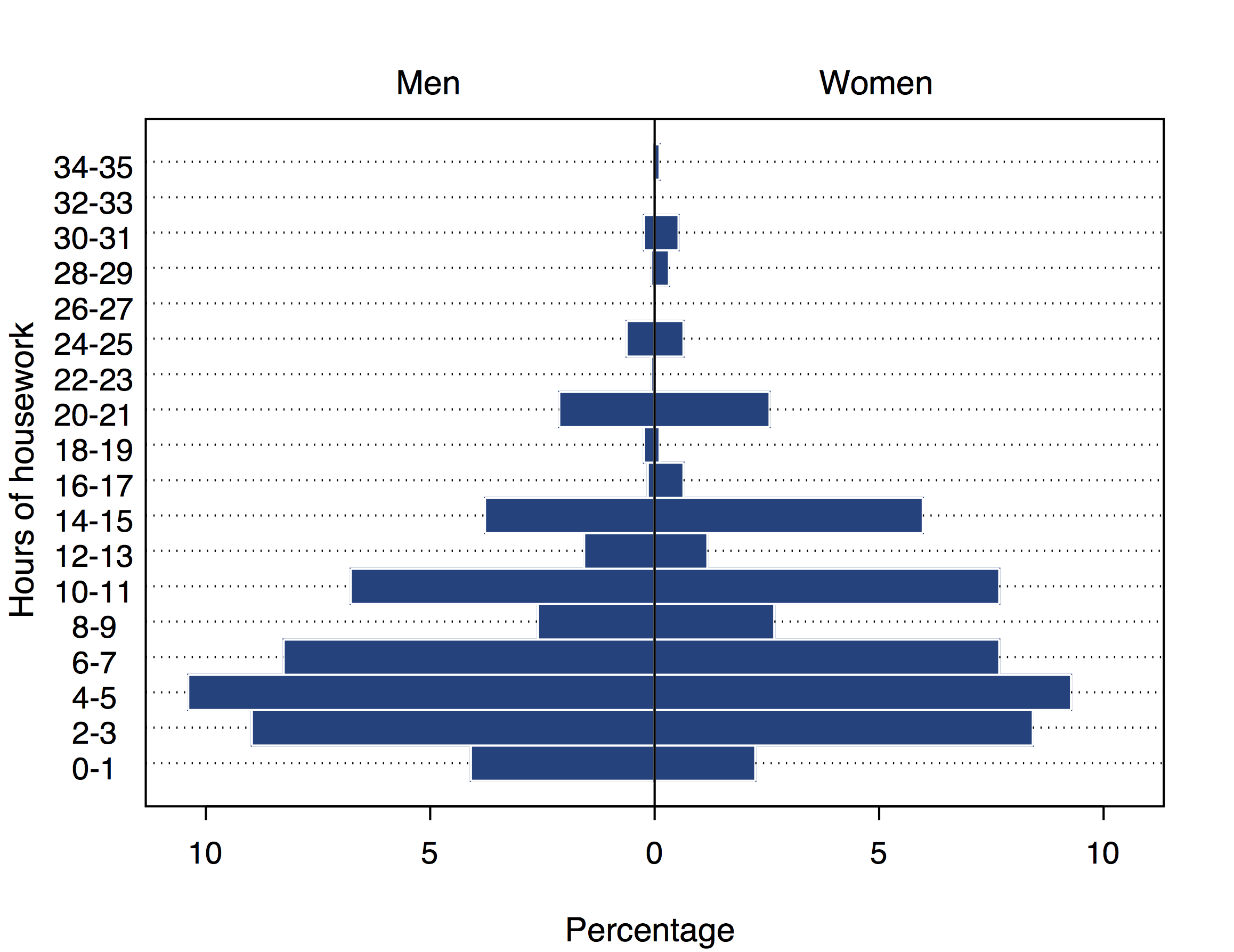
In Section 2.5.2 we described four graphical methods of summarizing the sample distribution of one continuous variable \(Y\): the histogram, the stem and leaf plot, the frequency polygon and the box plot. Each of these can be adapted for comparisons of two or more distributions, although some more conveniently than others. We illustrate the use three of the plots for this purpose, using the comparison of housework hours in Example 7.2 for illustration. Stem and leaf plots will not be shown, because they are less appropriate when the sample sizes are as large as they are in this example.

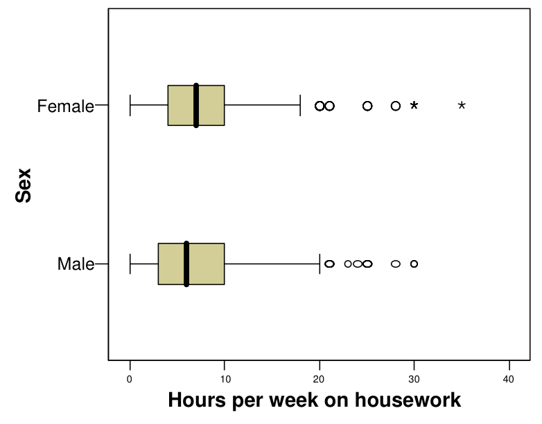
Two sample distributions can be compared by displaying histograms of them side by side, as shown in Figure 7.1. This is not a very common type of graph, and not ideal for visually comparing the two distributions, because the bars to be compared (here for men vs. women) end at opposite ends of the plot. A better alternative is to use frequency polygons. Since these represent a sample distribution by a single line, it is easy to include two of them in the same plot, as shown in Figure 7.2. Finally, Figure 7.3 shows two boxplots of reported housework hours, one for men and one for women.

The plots suggest that the distributions are quite similar for men and women. In both groups, the largest proportion of respondents stated that they do between 4 and 7 hours of housework a week. The distributions are clearly positively skewed, since the reported number of hours was much higher than average for a number of people (whereas less than zero hours were of course not recorded for anyone). The proportions of observations in categories including values 5, 10, 15, 20, 25 and 30 tend to be relatively high, suggesting that many respondents chose to report their answers in such round numbers. The box plots show that the median number of hours is higher for women than for men (7 vs. 6 hours), and women’s responses have slightly less variation, as measured by both the IQR and the range of the whiskers. Both distributions have several larger, outlying observations (note that SPSS, which was used to produce Figure 7.3, divides outliers into moderate and “extreme” ones; the latter are observations more than 3 IQR from the end of the box, and are plotted with asterisks).

Figure 7.1: Histograms of the sample distributions of reported weekly hours of housework in Example 7.2, separately for men (\(n=635\)) and women (\(n=469\)).

Figure 7.2: Frequency polygons of the sample distributions of reported weekly hours of housework in Example 7.2, separately for men and women. The points show the percentages of observations in the intervals of 0–3, 4–7, \(\dots\), 32–35 hours (plus zero percentages at each end of the curve).

Figure 7.3: Box plots of the sample distributions of reported weekly hours of housework in Example 7.2, separately for men and women.

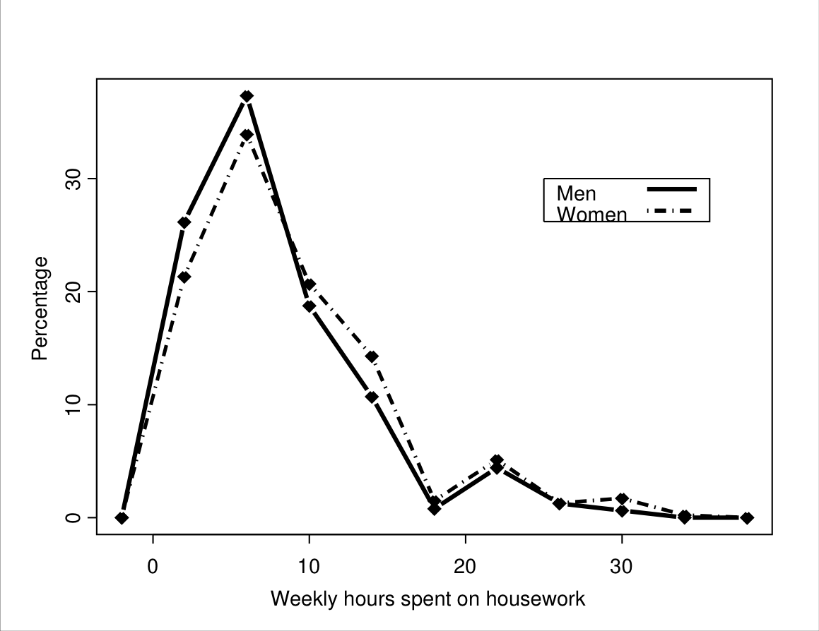
Figures 7.1–7.3 also illustrate an important general point about such comparisons. Typically we focus on comparing means of the conditional distributions. Here the difference between the sample means is 1.16, i.e. women in the sample spend, on average, over an hour longer on housework per week than men. The direction of the difference could also be guessed from Figure 7.2, which shows that somewhat smaller proportions of women than of men report small numbers of hours, and larger proportions of women report large numbers. This difference will later be shown to be statistically significant, and it is also arguably relatively large in a substantive sense.

However, it is equally important to note that the two distributions summarized by the graphs are nevertheless largely similar. For example, even though the mean is higher for women, there are clearly many women who report spending hardly any time on housework, and many men who spend a lot of time on it. In other words, the two distributions overlap to a large extent. This obvious point is often somewhat neglected in public discussions of differences between groups such as men and women or different ethnic groups. It is not uncommon to see reports of research indicating that (say) men have higher or lower values of something or other then women. Such statements usually refer to differences of averages, and are often clearly important and interesting. Less helpful, however, is the tendency to discuss the differences almost as if the corresponding distributions had no overlap at all, i.e. as if all men were higher or lower in some characteristic than all women. This is obviously hardly ever the case.

Box plots and frequency polygons can also be used to compare more than two sample distributions. For example, the experimental conditions in the study behind Example 7.3 actually involved not only whether or not a police officer wore sunglasses, but also whether or not he wore a gun. Distributions of perceived friendliness given all four combinations of these two conditions could easily be summarized by drawing four box plots or frequency polygons in the same plot, one for each experimental condition.

7.2.2 Comparing summary statistics

Main features of sample distributions, such as their central tendencies and variations, are described using the summary statistics introduced in Section 2.6. These too can be compared between groups. Table 7.1 shows such statistics for the examples of this chapter. Tables like these are routinely reported for initial description of data, even if more elaborate statistical methods are later used.

Sometimes the association between two variables in a sample is summarized in a single measure of association calculated from the data. This is especially convenient when both of the variables are continuous (in which case the most common measure of association is known as the correlation coefficient). In this section we consider as such a summary the difference \(\hat{\Delta}=\bar{Y}_{2}-\bar{Y}_{1}\) of the sample means of \(Y\) in the two groups. These differences are also shown in Table 7.1.

The difference of means is important because it is also the focus of the most common methods of inference for two-group comparisons. For purely descriptive purposes it may be as or more convenient to report some other statistic. For example, the difference of means of 1.16 hours in Example 7.2 could also be described in relative terms by saying that the women’s average is about 16 per cent higher than the men’s average (because \(1.16/7.33=0.158\), i.e. the difference represents 15.8 % of the men’s average).

7.3 Inference for two means from independent samples

7.3.1 Aims of the analysis

Formulated as a statistical model in the sense discussed on page in Section 6.3.1, the assumptions of the analyses considered in this section are as follows:

1. We have a sample of \(n_{1}\) independent observations of a variable \(Y\) in group 1, which have a population distribution with mean \(\mu_{1}\) and standard deviation \(\sigma_{1}\).

2. We have a sample of \(n_{2}\) independent observations of \(Y\) in group 2, which have a population distribution with mean \(\mu_{2}\) and standard deviation \(\sigma_{2}\).

3. The two samples are independent, in the sense discussed following Example 7.5.

4. For now, we further assume that the population standard deviations \(\sigma_{1}\) and \(\sigma_{2}\) are equal, with a common value denoted by \(\sigma\). This relatively minor assumption will be discussed further in Section 7.3.4.

We could have stated the starting points of the analyses in Chapters 4 and 5 also in such formal terms. It is not absolutely necessary to always do so, but we should at least remember that any statistical analysis is based on some such model. In particular, this helps to make it clear what our methods of analysis do and do not assume, so that we may critically examine whether these assumptions appear to be justified for the data at hand.

The model stated above does not require that the population distributions of \(Y\) should have the form of any particular probability distribution. It is often further assumed that these distributions are normal distributions, but this is not essential. Discussion of this question is postponed until Section 7.3.4.

The only new term in this model statement was the “independent” under assumptions 1 and 2. This statistical term can be roughly translated as “unrelated”. The condition can usually be regarded as satisfied when the units of analysis are different entities, as in Examples 7.2 and 7.3 where the units within each group are distinct individual people. In these examples the individuals in the two groups are also distinct, from which it follows that the two samples are independent as required by assumption 3. The same assumption of independent observations is also required by all of the methods described in Chapters 4 and 5, although we did not state this explicitly there.

This situation is illustrated by Example 7.2, where \(Y\) is the number of hours a person spends doing housework in a week, and the two groups are men (group 1) and women (group 2).

The quantity of main interest is here the difference of population means \[\begin{equation} \Delta=\mu_{2}-\mu_{1}. \tag{7.1} \end{equation}\] In particular, if \(\Delta=0\), the population means in the two groups are the same. If \(\Delta\ne 0\), they are not the same, which implies that there is an association between \(Y\) and the group in the population.

Inference on \(\Delta\) can be carried out using methods which are straightforward modifications of the ones introduced first in Chapter 5. For significance testing, the null hypothesis of interest is \[\begin{equation} H_{0}: \; \Delta=0, \tag{7.2} \end{equation}\] to be tested against a two-sided (\(H_{a}:\; \Delta\ne 0\)) or one-sided (\(H_{a}:\; \Delta> 0\) or \(H_{a}:\; \Delta< 0\)) alternative hypothesis. The test statistic used to test ((7.2)) is again of the form \[\begin{equation} t=\frac{\hat{\Delta}}{\hat{\sigma}_{\hat{\Delta}}} \tag{7.3} \end{equation}\] where \(\hat{\Delta}\) is a sample estimate of \(\Delta\), and \(\hat{\sigma}_{\hat{\Delta}}\) its estimated standard error. Here the statistic is conventionally labelled \(t\) rather than \(z\) and called the t-test statistic because sometimes the \(t\)-distribution rather than the normal is used as its sampling distribution. This possibility is discussed in Section 7.3.4, and we can ignore it until then.

Confidence intervals for the differences \(\Delta\) are also of the familiar form \[\begin{equation} \hat{\Delta} \pm z_{\alpha/2}\, \hat{\sigma}_{\hat{\Delta}} \tag{7.4} \end{equation}\] where \(z_{\alpha/2}\) is the appropriate multiplier from the standard normal distribution to obtain the required confidence level, e.g. \(z_{0.025}=1.96\) for 95% confidence intervals. The multiplier is replaced with a slightly different one if the \(t\)-distribution is used as the sampling distribution, as discussed in Section 7.3.4.

The details of these formulas in the case of two-sample inference on means are described next, in Section 7.3.2 for the significance test and in Section 7.3.3 for the confidence interval.

7.3.2 Significance testing: The two-sample t-test

For tests of the difference of means \(\Delta=\mu_{2}-\mu_{1}\) between two population distributions, we consider the null hypothesis of no difference \[\begin{equation} H_{0}: \; \Delta=0. \tag{7.5} \end{equation}\] In the housework example, this is the hypothesis that average weekly hours of housework in the population are the same for men and women. It is tested against an alternative hypothesis, either the two-sided alternative hypotheses \[\begin{equation} H_{a}: \; \Delta\ne 0 \tag{7.6} \end{equation}\] or one of the one-sided alternative hypotheses \[H_{a}: \Delta> 0 \text{ or } H_{a}: \Delta< 0\] In the discussion below, we concentrate on the more common two-sided alternative.

The test statistic for testing ((7.5)) is of the general form ((7.3)). Here it depends on the data only through the sample means \(\bar{Y}_{1}\) and \(\bar{Y}_{2}\) and sample variances \(s_{1}^{2}\) and \(s_{2}^{2}\) of \(Y\) in the two groups. A point estimate of \(\Delta\) is \[\begin{equation} \hat{\Delta}=\bar{Y}_{2}-\bar{Y}_{1}. \tag{7.7} \end{equation}\] In terms of the population parameters, the standard error of \(\hat{\Delta}\) is \[\begin{equation} \sigma_{\hat{\Delta}}=\sqrt{\sigma^{2}_{\bar{Y}_{2}}+\sigma^{2}_{\bar{Y}_{1}}}=\sqrt{\frac{\sigma^{2}_{2}}{n_{2}}+\frac{\sigma^{2}_{1}}{n_{1}}}. \tag{7.8} \end{equation}\] When we assume that the population standard deviations \(\sigma_{1}\) and \(\sigma_{2}\) are equal, with a common value \(\sigma\), ((7.8)) simplifies to \[\begin{equation} \sigma_{\hat{\Delta}} =\sigma\; \sqrt{\frac{1}{n_{2}}+\frac{1}{n_{1}}}. \tag{7.9} \end{equation}\] The formula of the test statistic uses an estimate of this standard error, given by \[\begin{equation} \hat{\sigma}_{\hat{\Delta}} =\hat{\sigma} \; \sqrt{\frac{1}{n_{2}}+\frac{1}{n_{1}}} \tag{7.10} \end{equation}\] where \(\hat{\sigma}\) is an estimate of \(\sigma\), calculated from \[\begin{equation} \hat{\sigma}=\sqrt{\frac{(n_{2}-1)s^{2}_{2}+(n_{1}-1)s^{2}_{1}}{n_{1}+n_{2}-2}}. \tag{7.11} \end{equation}\] Substituting ((7.7)) and ((7.10)) into the general formula ((7.3)) gives the two-sample t-test statistic for means \[\begin{equation} t=\frac{\bar{Y}_{2}-\bar{Y}_{1}} {\hat{\sigma}\, \sqrt{1/n_{2}+1/n_{1}}} \tag{7.12} \end{equation}\] where \(\hat{\sigma}\) is given by ((7.11)).

For an illustration of the calculations, consider again the housework Example 7.2. Here, denoting men by 1 and women by 2, \(n_{1}=635\), \(n_{2}=469\), \(\bar{Y}_{1}=7.33\), \(\bar{Y}_{2}=8.49\), \(s_{1}=5.53\) and \(s_{2}=6.14\). The estimated mean difference is thus \[\hat{\Delta}=\bar{Y}_{2}-\bar{Y}_{1}=8.49-7.33=1.16.\] The common value of the population standard deviation \(\sigma\) is estimated from ((7.11)) as \[\begin{aligned} \hat{\sigma}&=& \sqrt{\frac{(n_{2}-1)s^{2}_{2}+(n_{1}-1)s^{2}_{1}}{n_{1}+n_{2}-2}} = \sqrt{\frac{(469-1) 6.14^{2}+(635-1) 5.53^{2}}{635+469-2}}\\ &=& \sqrt{33.604}=5.797\end{aligned}\] and the estimated standard error of \(\hat{\Delta}\) is given by ((7.10)) as \[\hat{\sigma}_{\hat{\Delta}} = \hat{\sigma} \; \sqrt{\frac{1}{n_{2}}+\frac{1}{n_{1}}} =5.797 \; \sqrt{\frac{1}{469}+\frac{1}{635}}=0.353.\] The value of the t-test statistic ((7.12)) is then obtained as \[t=\frac{1.16}{0.353}=3.29.\] These values and other quantities explained later, as well as similar results for Example 7.3, are also shown in Table 7.3.

\(\hat{\Delta}\)	\(\hat{\sigma}_{\hat{\Delta}}\)	\(t\)	\(P\)-value	95 % C.I.
Example 7.2: Average weekly hours spent on housework
1.16	0.353	3.29	0.001	(0.47; 1.85)
Example 7.3: Perceived friendliness of a police officer
\(-1.74\)	0.383	\(-4.55\)	\(<0.001\)	\((-2.49; -0.99)\)

:(#tab:t-2testsY1)Results of tests and confidence intervals for comparing means for two independent samples. For Example 7.2, the difference of means is between women and men, and for Example 7.3, it is between wearing and not wearing sunglasses. The test statistics and confidence intervals are obtained under the assumption of equal population standard deviations, and the \(P\)-values are for a test with a two-sided alternative hypothesis. See the text for the definitions of the statistics.

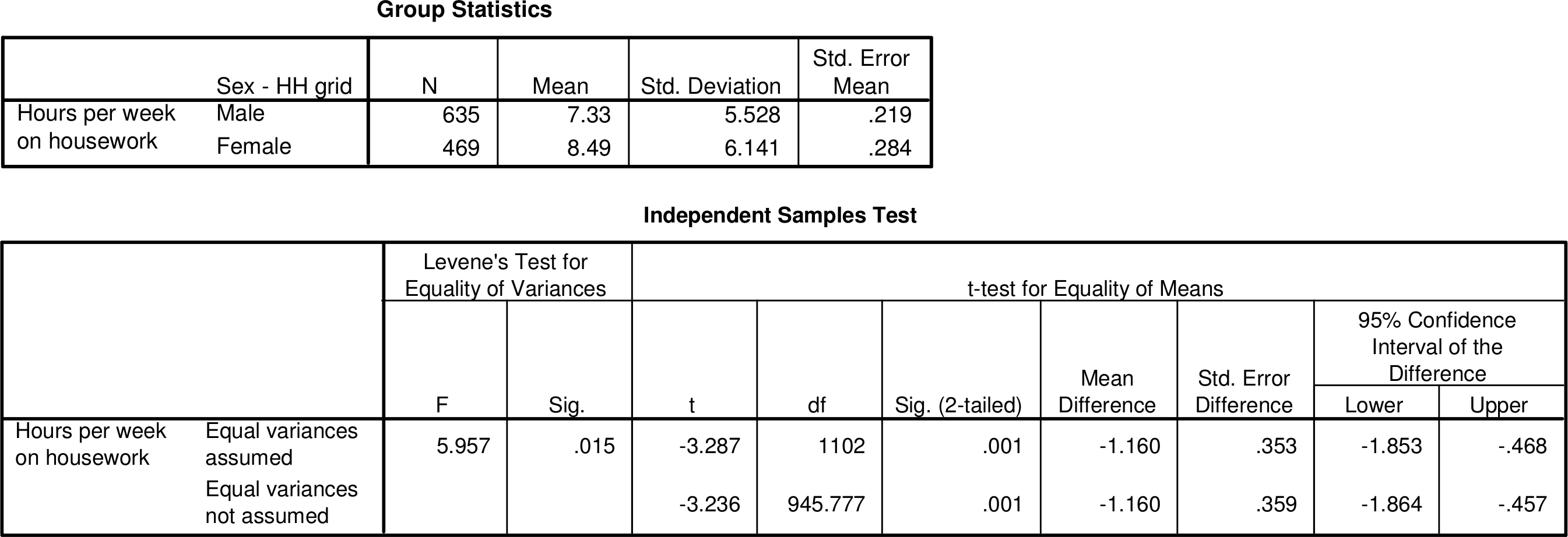
If necessary, calculations like these can be carried out even with a pocket calculator. It is, however, much more convenient to leave them to statistical software. Figure 7.4 shows SPSS output for the two-sample t-test for the housework data. The first part of the table, labelled “Group Statistics”, shows the sample sizes \(n\), means \(\bar{Y}\) and standard deviations \(s\) separately for the two groups. The quantity labelled “Std. Error Mean” is \(s/\sqrt{n}\). This is an estimate of the standard error of the sample mean, which is the quantity \(\sigma/\sqrt{n}\) discussed in Section 6.4.

The second part of the table in Figure 7.4, labelled “Independent Samples Test”, gives results for the t-test itself. The test considered here, which assumes a common population standard deviation \(\sigma\) (and thus also variance \(\sigma^{2}\)), is found on the row labelled “Equal variances assumed”. The test statistic is shown in the column labelled “\(t\)”, and the difference \(\hat{\Delta}=\bar{Y}_{2}-\bar{Y}_{1}\) and its standard error \(\hat{\sigma}_{\hat{\Delta}}\) are shown in the “Mean Difference” and “Std. Error Difference” columns respectively. Note that the difference (\(-1.16\)) has been calculated in SPSS between men and women rather than vice versa as in Table 7.3, but this will make no difference to the conclusions from the test.

Figure 7.4: SPSS output for a two-sample \(t\)-test in Example 7.2, comparing average weekly hours spent on housework between men and women.

In the two-sample situation with assumptions 1–4 at the beginning of Section 7.3.1, the sampling distribution of the t-test statistic ((7.12)) is approximately a standard normal distribution when the null hypothesis \(H_{0}: \; \Delta=\mu_{2}-\mu_{1}=0\) is true in the population and the sample sizes are large enough. This is again a consequence of the Central Limit Theorem. The requirement for “large enough” sample sizes is fairly easy to satisfy. A good rule of thumb is that the sample sizes \(n_{1}\) and \(n_{2}\) in the two groups should both be at least 20 for the sampling distribution of the test statistic to be well enough approximated by the standard normal distribution. In the housework example we have data on 635 men and 469 women, so the sample sizes are clearly large enough. A variant of the test which relaxes the condition on the sample sizes is discussed in Section 7.3.4 below.

The \(P\)-value of the test is calculated from this sampling distribution in exactly the same way as for the tests of proportions in Section 5.5.3. In the housework example the value of the \(t\)-test statistic is \(t=3.29\). The \(P\)-value for testing the null hypothesis against the two-sided alternative ((7.6)) is then the probability, calculated from the standard normal distribution, of values that are at least 3.29 or at most \(-3.29\). Each of these two probabilities is about 0.0005, so the \(P\)-value is \(0.0005+0.0005=0.001\). In the SPSS output of Figure 7.4 it is given in the column labelled “Sig. (2-tailed)”, where “Sig.” is short for “significance” and “2-tailed” is a synonym for “2-sided”.

The \(P\)-value can also be calculated approximately using the table of the standard normal distribution (see Table 5.2, as explained in Section 5.5.3. Here the test statistic \(t=3.29\), which is larger than the critical values 1.65, 1.96 and 2.58 for the 0.10, 0.05 and 0.01 significance levels for a two-sided test, so we can report that \(P<0.01\). Here \(t\) is by chance actually equal (to two decimal places) to the critical value for the 0.001 significance level, so we could also report \(P=0.001\). These findings agree, as they should, with the exact \(P\)-value of 0.001 shown in the SPSS output.

In conclusion, the two-sample \(t\)-test in Example 7.2 indicates that there is very strong evidence (with \(P=0.001\) for the two-sided test) against the claim that the hours of weekly housework are on average the same for men and women in the population.

Here we showed raw SPSS output in Figure 7.4 because we wanted to explain its contents and format. Note, however, that such unedited computer output is rarely if ever appropriate in research reports. Instead, results of statistical analyses should be given in text or tables formatted in appropriate ways for presentation. See Table 7.3 and various other examples in this coursepack and textbooks on statistics.

To summarise the elements of the test again, we repeat them briefly, now for Example 7.3, the experiment on the effect of eye contact on the perceived friendliness of police officers (c.f. Table 7.1 for the summary statistics):

1. Data: samples from two groups, one with the experimental condition where the officer wore no sunglasses, with sample size \(n_{1}=67\), mean \(\bar{Y}_{1}=8.23\) and standard deviation \(s_{1}=2.39\), and the second with the experimental condition where the officer did wear sunglasses, with \(n_{2}=66\), \(\bar{Y}_{2}=6.49\) and \(s_{2}=2.01\).

2. Assumptions: the observations are random samples of statistically independent observations from two populations, one with mean \(\mu_{1}\) and standard deviation \(\sigma_{1}\), and the other with with mean \(\mu_{2}\) and the same standard deviation \(\sigma_{2}\), where the standard deviations are equal, with value \(\sigma=\sigma_{1}=\sigma_{2}\). The sample sizes \(n_{1}\) and \(n_{2}\) are sufficiently large, say both at least 20, for the sampling distribution of the test statistic under the null hypothesis to be approximately standard normal.

3. Hypotheses: These are about the difference of the population means \(\Delta=\mu_{2}-\mu_{1}\), with null hypothesis \(H_{0}: \Delta=0\). The two-sided alternative hypothesis \(H_{a}: \Delta\ne 0\) is considered in this example.

4. The test statistic: the two-sample \(t\)-statistic \[t=\frac{\hat{\Delta}}{\hat{\sigma}_{\hat{\Delta}}}= \frac{-1.74}{0.383}=-4.55\] where \[\hat{\Delta}=\bar{Y}_{2}-\bar{Y}_{1}=6.49-8.23=-1.74\] and \[\hat{\sigma}_{\hat{\Delta}}= \hat{\sigma} \; \sqrt{\frac{1}{n_{2}}+\frac{1}{n_{1}}} =2.210 \times \sqrt{ \frac{1}{66}+\frac{1}{67}}=0.383\] with \[\hat{\sigma}= \sqrt{\frac{(n_{2}-1)s^{2}_{2}+(n_{1}-1)s^{2}_{1}}{n_{1}+n_{2}-2}} = \sqrt{\frac{65\times 2.01^{2}+66\times 2.39^{2}}{131}} =2.210\]

5. The sampling distribution of the test statistic when \(H_{0}\) is true: approximately the standard normal distribution.

6. The \(P\)-value: the probability that a randomly selected value from the standard normal distribution is at most \(-4.55\) or at least 4.55, which is about 0.000005 (reported as \(P<0.001\)).

7. Conclusion: A two-sample \(t\)-test indicates very strong evidence that the average perceived level of the friendliness of a police officer is different when the officer is wearing reflective sunglasses than when the officer is not wearing such glasses (\(P<0.001\)).

7.3.3 Confidence intervals for a difference of two means

A confidence interval for the mean difference \(\Delta=\mu_{1}-\mu_{2}\) is obtained by substituting appropriate expressions into the general formula ((7.4)). Specifically, here \(\hat{\Delta}=\bar{Y}_{2}-\bar{Y}_{1}\) and a 95% confidence interval for \(\Delta\) is \[\begin{equation} (\bar{Y}_{2}-\bar{Y}_{1}) \pm 1.96\; \hat{\sigma} \;\sqrt{\frac{1}{n_{2}}+\frac{1}{n_{1}}} \tag{7.13} \end{equation}\] where \(\hat{\sigma}\) is obtained from equation (7.11). The validity of this again requires that the sample sizes \(n_{1}\) and \(n_{2}\) from both groups are reasonably large, say both at least 20. For the housework Example 7.2, the 95% confidence interval is \[1.16\pm 1.96\times 0.353 = 1.16 \pm 0.69 = (0.47; 1.85)\] using the values of \(\bar{Y}_{2}-\bar{Y}_{1}\) and its standard error calculated earlier. This interval is also shown in Table 7.3 and in the SPSS output in Figure 7.4 . In the latter, the interval is given as (-1.85; -0.47) because it is expressed for the difference defined in the opposite direction (men \(-\) women instead of vice versa). For Example 7.3, the 95% confidence interval is \(-1.74\pm 1.96\times 0.383=(-2.49; -0.99)\).

Based on the data in Example 7.2 we are thus 95 % confident that the difference between women’s and men’s average hours of reported weekly housework in the population is between 0.47 and 1.85 hours. In substantive terms this interval, from just under half an hour to nearly two hours, is arguably fairly wide in that its two end points might well be regarded as substantially different from each other. The difference between women’s and men’s average housework hours is thus estimated fairly imprecisely from this survey.

7.3.4 Variants of the test and confidence interval

Allowing unequal population variances

The two-sample \(t\)-test and confidence interval for the difference of means were stated above under the assumption that the standard deviations \(\sigma_{1}\) and \(\sigma_{2}\) of the variable of interest \(Y\) are the same in both of the two groups being compared. This assumption is not in fact essential. If it is omitted, we obtain formulas which differ from the ones discussed above only in one part of the calculations.

Suppose that we do allow the unknown values of \(\sigma_{1}\) and \(\sigma_{2}\) to be different from each other. In other words, we consider the model stated at the beginning of Section 7.3.1, without assumption 4 that \(\sigma_{1}=\sigma_{2}\). The test statistic is then still of the same form as before, i.e. \(t=\hat{\Delta}/\hat{\sigma}_{\hat{\Delta}}\), with \(\hat{\Delta}=\bar{Y}_{2}-\bar{Y}_{1}\). The only change in the calculations is that the estimate of the standard error of \(\hat{\Delta}\), the formula of which is given by equation ((7.8)), now uses separate estimates of \(\sigma_{1}\) and \(\sigma_{2}\). The obvious choices for these are the corresponding sample standard deviations, \(s_{1}\) for \(\sigma_{1}\) and \(s_{2}\) for \(\sigma_{2}\). This gives the estimated standard error as \[\begin{equation} \hat{\sigma}_{\hat{\Delta}}=\sqrt{\frac{s_{2}^{2}}{n_{2}}+\frac{s_{1}^{2}}{n_{1}}}. \tag{7.14} \end{equation}\] Substituting this to the formula of the test statistic yields the two-sample \(t\)-test statistic without the assumption of equal population standard deviations, \[\begin{equation} t=\frac{\bar{Y}_{2}-\bar{Y}_{1}}{\sqrt{s^{2}_{2}/n_{2}+s^{2}_{1}/n_{1}}}. \tag{7.15} \end{equation}\] The sampling distribution of this under the null hypothesis is again approximately a standard normal distribution when the sample sizes \(n_{1}\) and \(n_{2}\) are both at least 20. The \(P\)-value for the test is obtained in exactly the same way as before, and the principles of interpreting the result of the test are also unchanged.

For the confidence interval, the only change from Section 7.3.3 is again that the estimated standard error is changed, so for a 95% confidence interval we use \[\begin{equation} (\bar{Y}_{2}-\bar{Y}_{1}) \pm 1.96 \;\sqrt{\frac{s^{2}_{2}}{n_{2}}+\frac{s^{2}_{1}}{n_{1}}}. \tag{7.16} \end{equation}\] In the housework example 7.2, the estimated standard error ((7.14)) is \[\hat{\sigma}_{\hat{\Delta}}= \sqrt{ \frac{6.14^{2}}{469}+ \frac{5.53^{2}}{635} }= \sqrt{0.1285}=0.359,\] the value of the test statistic is \[t=\frac{1.16}{0.359}=3.23,\] and the two-sided \(P\)-value is now \(P=0.001\). Recall that when the population standard deviations were assumed to be equal, we obtained \(\hat{\sigma}_{\hat{\Delta}}=0.353\), \(t=3.29\) and again \(P=0.001\). The two sets of results are thus very similar, and the conclusions from the test are the same in both cases. The differences between the two variants of the test are even smaller in Example 7.3, where the estimated standard error \(\hat{\sigma}_{\hat{\Delta}}=0.383\) is the same (to three decimal places) in both cases, and the results are thus identical.³³ In both examples the confidence intervals obtained from ((7.13)) and ((7.16)) are also very similar. Both variants of the two-sample analyses are shown in SPSS output (c.f. Figure 7.4), the ones assuming equal population standard deviations on the row labelled “Equal variances assumed” and the one without this assumption on the “Equal variances not assumed” row.³⁴

Which methods should we then use, the ones with or without the assumption of equal population variances? In practice the choice rarely makes much difference, and the \(P\)-values and conclusions from the two versions of the test are typically very similar.³⁵ Not assuming the variances to be equal has the advantage of making fewer restrictive assumptions about the population. For this reason it should be used in the rare cases where the \(P\)-values obtained under the different assumptions are substantially different. This version of the test statistic is also slightly easier to calculate by hand, since ((7.14)) is a slightly simpler formula than ((7.10))–((7.11)). On the other hand, the test statistic which does assume equal standard deviations has the advantage that it is more closely related to analogous tests used in more general contexts (especially the method of linear regression modelling, discussed in Chapter 8). It is also preferable when the sample sizes are very small, as discussed below.

Using the \(t\) distribution

As discussed in Section 6.3, it is often assumed that the population distributions of the variables under consideration are described by particular probability distributions. In this chapter, however, such assumptions have so far been avoided. This is a consequence of the Central Limit Theorem, which ensures that as long as the sample sizes are large enough, the sampling distribution of the two-sample \(t\)-test statistic is approximately the standard normal distribution, irrespective of the forms of the population distributions of \(Y\) in the two groups. In this section we briefly describe variants of the test and confidence interval which do assume that the population distributions are of a particular form, specifically that they are normal distributions. This changes the sampling distribution that is used for the test statistic and for the multiplier of the confidence interval, but the analyses are otherwise unchanged.

For the significance test, there are again two variants depending on the assumptions about the the population standard deviations \(\sigma_{1}\) and \(\sigma_{2}\). Consider first the case where these are assumed to be equal. The sampling distribution is then given by the following result, which now holds for any sample sizes \(n_{1}\) and \(n_{2}\):

• In the two-sample situation specified by assumptions 1–4 at the beginning of Section 7.3.1 (including the assumption of equal population standard deviations, \(\sigma_{1}=\sigma_{2}=\sigma\)), and if also the distribution of \(Y\) is a normal distribution in both groups, the sampling distribution of the t-test statistic ((7.12)) is a \(t\) distribution with \(n_{1}+n_{2}-2\) degrees of freedom when the null hypothesis \(H_{0}: \; \Delta=\mu_{2}-\mu_{1}=0\) is true in the population.

The \(\mathbf{t}\) distributions mentioned in this result are a family of distributions with different degrees of freedom, in a similar way as the \(\chi^{2}\) distributions discussed in Section 4.3.4. All \(t\) distributions are symmetric around 0. Their shape is quite similar to that of the standard normal distribution, except that the variance of a \(t\) distribution is somewhat larger and its tails thus heavier. The difference is noticeable only when the degrees of freedom are small, as seen in Figure 7.5. This shows the curves for the \(t\) distributions with 6 and 30 degrees of freedom, compared to the standard normal distribution. It can be seen that the \(t_{30}\) distribution is already very similar to the \(N(0,1)\) distribution. With degrees of freedom larger than about 30, the difference becomes almost indistinguishable.

Figure 7.5: Curves of two \(t\) distributions with small degrees of freedom, compared to the standard normal distribution.

If we use this result for the test, the \(P\)-value is obtained from the \(t\) distribution with \(n_{1}+n_{2}-2\) degrees of freedom (often denoted \(t_{n1+n2-2}\)). The principles of doing this are exactly the same as those described in Section 5.5.3, and can be graphically illustrated by plots similar to those in Figure 5.1. Precise \(P\)-values are again obtained using a computer. In fact, \(P\)-values in SPSS output for the two-sample \(t\)-test (c.f. Figure 7.4) are actually those obtained from the \(t\) distribution (with the degrees of freedom shown in the column labelled “df”) rather than the standard normal distribution. Differences between the two are, however, very small if the sample sizes are even moderately large, because then the degrees of freedom \(df=n_{1}+n_{2}-2\) are large enough for the two distributions to be virtually identical. This is the case, for instance, in both of the examples considered so far in this chapter, where \(df=1102\) in Example 7.2 and \(df=131\) in Example 7.3.

If precise \(P\)-values from the \(t\) distribution are not available, upper bounds for them can again be obtained using appropriate tables, in the same way as in Section 5.5.3. Now, however, the critical values depend also on the degrees of freedom. Because of this, introductory text books on statistics typically include a table of critical values for \(t\) distributions for a selection of degrees of freedom. A table of this kind is shown in the Appendix at the end of this course pack. Each row of the table corresponds to a \(t\) distribution with the degrees of freedom given in the column labelled “df”. As here, such tables typically include all degrees of freedom between 1 and 30, plus a selection of larger values, here 40, 60 and 120.

The last row is labelled “\(\infty\)”, the mathematical symbol for infinity. This corresponds to the standard normal distribution, as a \(t\) distribution with infinite degrees of freedom is equal to the standard normal. The practical implication of this is that the standard normal distribution is a good enough approximation for any \(t\) distribution with reasonably large degrees of freedom. The table thus lists individual degrees of freedom only up to some point, and the last row will be used for any values larger than this. For degrees of freedom between two values shown in the table (e.g. 50 when only 40 and 60 are given), it is best to use the values for the nearest available degrees of freedom below the required ones (e.g. use 40 for 50). This will give a “conservative” approximate \(P\)-value which may be slightly larger than the exact value.

As for the standard normal distribution, the table is used to identify critical values for different significance levels (c.f. the information in Table 5.2). For example, if the degrees of freedom are 20, the critical value for two-sided tests at the significance level 0.05 in the “0.025” column on the row labelled “20”. This is 2.086. In general, critical values for \(t\) distributions are somewhat larger than corresponding values for the standard normal distribution, but the difference between the two is quite small when the degrees of freedom are reasonably large.

The \(t\)-test and the \(t\) distribution are among the oldest tools of statistical inference. They were introduced in 1908 by W. S. Gosset,³⁶ initially for the one-sample case discussed in Section 7.4. Gosset was working as a chemist at the Guinness brewery at St. James’ Gate, Dublin. He published his findings under the pseudonym “Student”, and the distribution is often known as Student’s \(t\) distribution.

These results for the sampling distribution hold when the population standard deviations \(\sigma_{1}\) and \(\sigma_{2}\) are assumed to be equal. If this assumption is not made, the test statistic is again calculated using formulas ((7.14)) and ((7.15)). This case is mathematically more difficult than the previous one, because the sampling distribution of the test statistic under the null hypothesis is then not exactly a \(t\) distribution even when the population distributions are normal. One way of dealing with this complication (which is known as the Behrens–Fisher problem) is to find a \(t\) distribution which is a good approximation of the true sampling distribution. The degrees of freedom of this approximating distribution are given by \[\begin{equation} df=\frac{\left(\frac{s^{2}_{1}}{n_{1}}+\frac{s^{2}_{2}}{n_{2}}\right)^{2}}{\left(\frac{s_{1}^{2}}{n_{1}}\right)^{2}\;\left(\frac{1}{n_{1}-1}\right)+\left(\frac{s_{2}^{2}}{n_{2}}\right)^{2}\;\left(\frac{1}{n_{2}-1}\right)}. \tag{7.17} \end{equation}\] This formula, which is known as the Welch-Satterthwaite approximation, is not particularly interesting or worth learning in itself. It is presented here purely for completeness, and to give an idea of how the degrees of freedom given in the SPSS output are obtained. In Example 7.2 (see Figure 7.4) these degrees of freedom are 945.777, showing that the approximate degrees of freedom from ((7.17)) are often not whole numbers. If approximate \(P\)-values are then obtained from a \(t\)-table, we need to use values for the nearest whole-number degrees of freedom shown in the table. This problem does not arise if the calculations are done with a computer.

Two sample \(t\)-test statistics (in two variants, under equal and unequal population standard deviations) have now been defined under two different sets of assumptions about the population distributions. In each case, the formula of the test statistic is the same, so the only difference is in the form of its sampling distribution under the null hypothesis. If the population distributions of \(Y\) in the two groups are assumed to be normal, the sampling distribution of the \(t\)-statistic is a \(t\) distribution with appropriate degrees of freedom. If the sample sizes are reasonably large, the sampling distribution is approximately standard normal, whatever the shape of the population distribution. Which set of assumptions should we then use? The following guidelines can be used to make the choice:

• The easiest and arguably most common case is the one where both sample sizes \(n_{1}\) and \(n_{2}\) are large enough (both greater than 20, say) for the standard normal approximation of the sampling distribution to be reasonably accurate. Because the degrees of freedom of the appropriate \(t\) distribution are then also large, the two sampling distributions are very similar, and conclusions from the test will be similar in either case. It is then purely a matter of convenience which sampling distribution is used:

  • If you use a computer (e.g. SPSS) to carry out the test or you are (e.g. in an exam) given computer output, use the \(P\)-value in the output. This will be from the \(t\) distribution.

  • If you need to calculate the test statistic by hand and thus need to use tables of critical values to draw the conclusion, use the critical values for the standard normal distribution (see Table 5.2).

• When the sample sizes are small (e.g. if one or both of them are less than 20), only the \(t\) distribution can be used, and even then only if \(Y\) is approximately normally distributed in both groups in the population. For some variables (say weight or blood pressure) we might have some confidence that this is the case, perhaps from previous, larger studies. In other cases the normality of \(Y\) can only be assessed based on its sample distribution, which of course is not very informative when the sample is small. In most cases, some doubt will remain, so the results of a \(t\)-test from small samples should be treated with caution. An alternative is then to use nonparametric tests which avoid the assumption of normality, for example the so-called Wilcoxon–Mann–Whitney test. These, however, are not covered on this course.

There are also situations where the population distribution of \(Y\) cannot possibly be normal, so the possibility of referring to a \(t\) distribution does not arise. One example are the tests on population proportions that were discussed in Chapter 5. There the only possibility we discussed was to use the approximate standard normal sampling distribution, as long as the sample sizes were large enough. Because the \(t\)-distribution is never relevant there, the test statistic is conventionally called the \(z\)-test statistic rather than \(t\). Sometimes the label \(z\) instead of \(t\) is used also for two-sample \(t\)-statistics described in this chapter. This does not change the test itself.

It is also possible to obtain a confidence interval for \(\Delta\) which is valid for even very small sample sizes \(n_{1}\) and \(n_{2}\), but only under the further assumption that the population distribution of \(Y\) in both groups is normal. This affects only the multiplier of the standard errors, which is now based on a \(t\) distribution. The appropriate degrees of freedom are again \(df=n_{1}+n_{2}-2\) when the population standard deviations are assumed equal, and approximately given by equation ((7.17)) if not. In this case the multiplier in ((7.4)) may be labelled \(t^{(df)}_{\alpha/2}\) instead of \(z_{\alpha/2}\) to draw attention to the fact that it comes from a \(t\)-distribution and depends on the degrees of freedom \(df\) as well as the significance level \(1-\alpha\).

Any multiplier \(t_{\alpha/2}^{(df)}\) is obtained from the relevant \(t\) distribution using exactly the same logic as the one explained for the normal distribution in the previous section, using a computer or a table of \(t\) distributions. For example, in the \(t\) table in the Appendix, multipliers for a 95% confidence interval are the numbers given in the column labelled “0.025”. Suppose, for instance, that the sample sizes \(n_{1}\) and \(n_{2}\) are both 10 and population standard deviations are assumed equal, so that \(df=10+10-2=18\). The table shows that a \(t\)-based 95% confidence interval would then use the multiplier 2.101. This is somewhat larger than the corresponding multiplier 1.96 from the normal distribution, and the \(t\)-based interval is somewhat wider than one based on the normal distribution. The difference between the two becomes very small when the sample sizes are even moderately large, because then \(df\) is large and \(t_{\alpha/2}^{(df)}\) is very close to 1.96.

The choice between confidence intervals based on the normal or a \(t\) distribution involves the same considerations as for the significance test. In short, if the sample sizes are not very small, the choice makes little difference and can be based on convenience. If you are calculating an interval by hand, a normal-based one is easier to use because the multiplier (e.g. 1.96 for 95% intervals) does not depend on the sample sizes. If, instead, a computer is used, it typically gives confidence intervals for differences of means based on the \(t\) distribution, so these are easier to use. Finally, if one or both of the sample sizes are small, only \(t\)-based intervals can safely be used, and then only if you are confident that the population distributions of \(Y\) are approximately normal.

7.4 Tests and confidence intervals for a single mean

The task considered in this section is inference on the population mean of a continuous, interval-level variable \(Y\) in a single population. This is thus analogous to the analysis of a single proportion in Sections 5.5–5.6, but with a continuous variable of interest.

We use Example 7.1 on survey data on diet for illustration. We will consider two variables, daily consumption of portions of fruit and vegetables, and the percentage of total faily energy intake obtained from fat and fatty acids. These will be analysed separately, each in turn in the role of the variable of interest \(Y\). Summary statistics for the variables are shown in Table 7.4

\(P\)-value \(P\)-value \

Two- One- 95% CI

Variable \(n\) \(\bar{Y}\) \(s\) \(\mu_{0}\) \(t\) sided\(^{*}\) sided\(^{\dagger}\) for \(\mu\)

Fruit and vegetable 1724 2.8 2.15 5 -49.49 \(<0.001\) \(<0.001\) (2.70; 2.90) consumption (400g portions)

Total energy intake 1724 35.3 6.11 35 2.04 0.042 0.021 (35.01; 35.59) from fat (%) —————————————————————————————————————————————

:(#tab:t-ttests1)Summary statistics, \(t\)-tests and confidence intervals for the mean for the two variables in Example 7.1 (variables from the Diet and Nutrition Survey). \(n=\)sample size; \(\bar{Y}=\)sample mean; \(s=\)sample standard deviation; \(\mu_{0}=\)null hypothesis about the population mean; \(t=t\)-test statistic; \(*\): Alternative hypothesis \(H_{a}: \mu\ne \mu_{0}\); \(\dagger\): Alternative hypotheses \(H_{a}: \mu<5\) and \(\mu>35\) respectively.

The setting for the analysis of this section is summarised as a statistical model for observations of a variable \(Y\) as follows:

1. The population distribution of \(Y\) has some unknown mean \(\mu\) and unknown standard deviation \(\sigma\).

2. The observations \(Y_{1}, Y_{2}, \dots, Y_{n}\) in the sample are a random sample from the population.

3. The observations are statistically independent, as discussed at the beginning of Section 7.3.1.

It is not necessary to assume that the population distribution has a particular form. However, this is again sometimes assumed to be a normal distribution, in which case the analyses may be modified in ways discussed below.

The only quantity of interest considered here is \(\mu\), the population mean of \(Y\). In the diet examples this is the mean number of portions of fruit and vegetables, or mean percentage of energy derived from fat (both on an average day for an individual) among the members of the population (which for this survey is British adults aged 19–64).

Because no separate groups are being compared, questions of interest are now not about differences between different group means, but about the value of \(\mu\) itself. The best single estimate (point estimate) of \(\mu\) is the sample mean \(\bar{Y}\). More information is provided by a confidence interval which shows which values of \(\mu\) are plausible given the observed data.

Significance testing focuses on the question of whether it is plausible that the true value of \(\mu\) is equal to a particular value \(\mu_{0}\) specified by the researcher. The specific value of \(\mu_{0}\) to be tested is suggested by the research questions. For example, we will consider \(\mu_{0}=5\) for portions of fruit and vegetables and \(\mu_{0}=35\) for the percentage of energy from fat. These values are chosen because they correspond to recommendations by the Department of Health that we should consume at least 5 portions of fruit and vegetables a day, and that fat should contribute no more than 35% of total energy intake. The statistical question is thus whether the average level of consumption in the population is at the recommended level.

In this setting, the null hypothesis for a significance test will be of the form \[\begin{equation} H_{0}: \; \mu=\mu_{0}, \tag{7.18} \end{equation}\] i.e. it claims that the unknown population mean \(\mu\) is equal to the value \(\mu_{0}\) specified by the null hypothesis. This will be tested against the two-sided alternative hypothesis \[\begin{equation} H_{a}: \; \mu\ne \mu_{0} \tag{7.19} \end{equation}\] or one of the one-sided alternative hypotheses \[\begin{equation} H_{a}: \mu> \mu_{0} \tag{7.20} \end{equation}\] or \[\begin{equation} H_{a}: \mu< \mu_{0}. \tag{7.21} \end{equation}\] For example, we might consider the one-sided alternative hypotheses \(H_{a}:\; \mu<5\) for portions of fruit and vegetables and \(H_{a}:\;\mu>35\) for the percentage of energy from fat. For both of these, the alternative corresponds to a difference from \(\mu_{0}\) in the unhealthy direction, i.e. less fruit and vegetables and more fat than are recommended.

To establish a connection to the general formulas that have been stated previously, it is again useful to express these hypotheses in terms of \[\begin{equation} \Delta=\mu-\mu_{0}, \tag{7.22} \end{equation}\] i.e. the difference between the unknown true mean \(\mu\) and the value \(\mu_{0}\) claimed by the null hypothesis. Because this is 0 if and only if \(\mu\) and \(\mu_{0}\) are equal, the null hypothesis ((7.18)) can also be expressed as \[\begin{equation} H_{0}: \; \Delta=0, \tag{7.23} \end{equation}\] and possible alternative hypotheses as \[\begin{equation} H_{0}: \Delta\ne0, \tag{7.24} \end{equation}\] \[\begin{equation} H_{0}: \Delta>0 \tag{7.25} \end{equation}\] and \[\begin{equation} H_{0}: \Delta< 0, \tag{7.26} \end{equation}\] corresponding to ((7.19)), ((7.20)) and ((7.21)) respectively.

The general formulas summarised in Section 7.3.1 can again be used, as long as their details are modified to apply to \(\Delta\) defined as \(\mu-\mu_{0}\). The resulting formulas are listed briefly below, and then illustrated using the data from the diet survey:

• The point estimate of the difference \(\Delta=\mu-\mu_{0}\) is \[\begin{equation} \hat{\Delta}=\bar{Y}-\mu_{0}. \tag{7.27} \end{equation}\]

• The standard error of \(\hat{\Delta}\), i.e. the standard deviation of its sampling distribution, is \(\sigma_{\hat{\Delta}}=\sigma/\sqrt{n}\) (note that this is equal to the standard error \(\sigma_{\bar{Y}}\) of the sample mean \(\bar{Y}\) itself).³⁷ This is estimated by \[\begin{equation} \hat{\sigma}_{\hat{\Delta}} = \frac{s}{\sqrt{n}}. \tag{7.28} \end{equation}\]

• The \(t\)-test statistic for testing the null hypothesis ((7.23)) is \[\begin{equation} t=\frac{\hat{\Delta}}{\hat{\sigma}_{\hat{\Delta}}} = \frac{\bar{Y}-\mu_{0}}{s/\sqrt{n}}. \tag{7.29} \end{equation}\]

• The sampling distribution of the \(t\)-statistic, when the null hypothesis is true, is approximately a standard normal distribution, when the sample size \(n\) is reasonably large. A common rule of thumb is that this sampling distribution is adequate when \(n\) is at least 30.

  • Alternatively, we may make the further assumption that the population distribution of \(Y\) is normal, in which case no conditions on \(n\) are required. The sampling distribution of \(t\) is then a \(t\) distribution with \(n-1\) degrees of freedom. The choice of which sampling distribution to refer to is based on the considerations outlined in Section 7.3.4. When \(n\) is 30 or larger, the two approaches give very similar results.

• \(P\)-values are obtained and the conclusions drawn in the same way as for two-sample tests, with appropriate modifications to the wording of the conclusions.

• A confidence interval for \(\Delta\), with confidence level \(1-\alpha\) and based on the approximate normal sampling distribution, is given by \[\begin{equation} \hat{\Delta}\pm z_{\alpha/2}\, \hat{\sigma}_{\hat{\Delta}} = (\bar{Y}-\mu_{0}) \pm z_{\alpha/2} \, \frac{s}{\sqrt{n}} \tag{7.30} \end{equation}\] where \(z_{\alpha/2}\) is the multiplier from the standard normal distribution for the required significance level (see Table 5.3), most often 1.96 for a 95% confidence interval. If an interval based on the \(t\) distribution is wanted instead, \(z_{\alpha/2}\) is replaced by the corresponding multiplier \(t_{\alpha/2}^{(n-1)}\) from the \(t_{n-1}\) distribution.

  Instead of the interval ((7.30)) for the difference \(\Delta=\mu-\mu_{0}\), it is usually more sensible to report a confidence interval for \(\mu\) itself. This is given by \[\begin{equation} \bar{Y} \pm z_{\alpha/2} \, \frac{s}{\sqrt{n}}, \tag{7.31} \end{equation}\] which is obtained by adding \(\mu_{0}\) to both end points of ((7.30)).

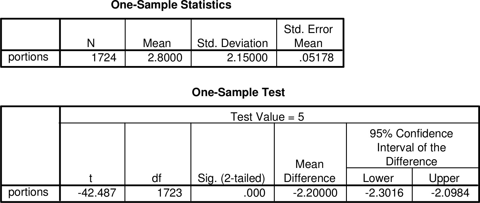
For the fruit and vegetable variable in the diet example, the mean under the null hypothesis is the dietary recommendation \(\mu_{0}=5\). The estimated difference ((7.27)) is \[\hat{\Delta}=2.8-5=-2.2\] and its estimated standard error ((7.28)) is \[\hat{\sigma}_{\hat{\Delta}}= \frac{2.15}{\sqrt{1724}} = 0.05178,\] so the \(t\)-test statistic ((7.29)) is \[t=\frac{-2.2}{0.05178} = -42.49.\] To obtain the \(P\)-value for the test, \(t=-42.49\) is referred to the sampling distribution under the null hypothesis, which can here be taken to be the standard normal distribution, as the sample size \(n=1723\) is large. If we consider the two-sided alternative hypothesis \(H_{a}:\; \Delta\ne 0\) (i.e. \(H_{a}:\; \mu\ne5\)), the \(P\)-value is the probability that a randomly selected value from the standard normal distribution is at most \(-42.49\) or at least 42.49. This is a very small probability, approximately \(0.00\cdots019\), with 268 zeroes between the decimal point and the 1. This is, of course, to all practical purposes zero, and can be reported as \(P<0.001\). The null hypothesis \(H_{0}:\; \mu=5\) is rejected at any conventional level of significance. A \(t\)-test for the mean indicates very strong evidence that the average daily number of portions of fruit and vegetables consumed by members of the population differs from the recommended minimum of five.

If we considered instead the one-sided alternative hypothesis \(H_{a}:\;\Delta<0\) (i.e. \(H_{a}: \; \mu<5\)), the observed sample mean \(\bar{Y}=2.8<5\) is in the direction of this alternative. The \(P\)-value is then the one-sided \(P\)-value divided by 2, which is here a small value reported as \(P<0.001\) again. The null hypothesis \(H_{0}: \; \mu=5\) (and by implication also the one-sided null hypothesis \(H_{0}:\; \mu\ge 5\), as discussed at the end of Section 5.5.1) is thus also rejected in favour of this one-sided alternative, at any conventional significance level.

A 95% confidence interval for \(\mu\) is obtained from ((7.31)) as \[2.8\pm 1.96 \times \frac{2.15}{\sqrt{1724}} =2.8\pm 1.96 \times 0.05178= 2.8\pm 0.10 = (2.70; 2.90).\] We are thus 95% confident that the average daily number of portions of fruit and vegetables consumed by members of the population is between 2.70 and 2.90.

Figure 7.6 shows how these results for the fruit and vegetable variable are displayed in SPSS output. The label “portions” refers to the name given to the variable in the SPSS data file, and “Test Value = 5” indicates the null hypothesis value \(\mu_{0}\) being tested. Other parts of the SPSS output correspond to the information in Table 7.4 in fairly obvious ways, so “N” indicates the sample size \(n\) (and not a population size, which is denoted by \(N\) in our notation), “Mean” the sample mean \(\bar{Y}\), “Std. Deviation” the sample standard deviation \(s\), “Std. Error Mean” the estimate of the standard error of the mean given by \(s/\sqrt{n}=2.15/\sqrt{1724}=0.05178\), “Mean Difference” the difference \(\hat{\Delta}=\bar{Y}-\mu_{0}=2.8-5=-2.2\), and “t” the \(t\)-test statistic ((7.29)). The \(P\)-value against the two-sided alternative hypothesis is shown as “Sig. (2-tailed)” (reported in the somewhat sloppy SPSS manner as “.000”). This is actually obtained from the \(t\) distribution, the degrees of freedom of which (\(n-1=1723\)) are given under “df”. Finally, the output also contains a 95% confidence interval for the difference \(\Delta=\mu-\mu_{0}\), i.e. the interval ((7.30)).³⁸ This is given as \((-2.30; -2.10)\). To obtain the more convenient confidence interval ((7.31)) for \(\mu\) itself, we only need to add \(\mu_{0}=5\) to both end points of the interval shown by SPSS, to obtain \((-2.30+5; -2.10+5)=(2.70; 2.90)\) as before.

Figure 7.6: SPSS output for a \(t\)-test of a single mean. The output is for the variable on fruit and vegetable consumption in Table 7.4, with the null hypothesis \(H-{0}: \mu=5\).

Similar results for the variable on the percentage of dietary energy obtained from fat are also shown in Table 7.4. Here \(\mu_{0}=35\), \(\hat{\Delta}=35.3-35=0.3\), \(\hat{\sigma}_{\hat{\Delta}}=6.11/\sqrt{1724}=0.147\), \(t=0.3/0.147\), and the two-sided \(P\)-value is \(P=0.042\). Here \(P<0.05\), so null hypothesis that the population average of the percentage of energy obtained from fat is 35 is rejected at the 5% level of significance. However, because \(P>0.01\), the hypothesis would not be rejected at the next conventional significance level of 1%. The conclusions are the same if we considered the one-sided alternative hypothesis \(H_{a}:\; \mu>35\), for which \(P=0.042/2=0.021\) (as the observed sample mean \(\bar{Y}=35.3\) is in the direction of \(H_{a}\)). In this case the evidence against the null hypothesis is thus somewhat less strong than for the fruit and vegetable variable, for which the \(P\)-value was extremely small. The 95% confidence interval for the population average of the fat variable is \(35.3\pm 1.96\times 0.147=(35.01; 35.59)\).

Analysis of a single population mean is a good illustration of some of the advantages of confidence intervals over significance tests. First, a confidence interval provides a summary of all the plausible values of \(\mu\) even when, as is very often the case, there is no obvious single value \(\mu_{0}\) to be considered as the null hypothesis of the one-sample \(t\)-test. Second, even when such a significance test is sensible, the conclusion can also be obtained from the confidence interval, as discussed at the end of Section 5.6.4. In other words, \(H_{0}:\; \mu=\mu_{0}\) is rejected at a given significance level against a two-sided alternative hypothesis, if the confidence interval for \(\mu\) at the corresponding confidence level does not contain \(\mu_{0}\), and not rejected if the interval contains \(\mu_{0}\). Here the 95% confidence interval (2.70; 2.90) does not contain 5 for the fruit and vegetable variable, and the interval (35.01; 35.59) does not contain 35 for the fat variable, so the null hypotheses with these values as \(\mu_{0}\) are rejected at the 5% level of significance.

The width of a confidence interval also gives information on how precise the results of the statistical analysis are. Here the intervals seem quite narrow for both variables, in that it seems that their end points (e.g. 2.7 and 2.9 for portions of fruit and vegetables) would imply qualitatively similar conclusions about the level of consumption in the population. Analysis of the sample of 1724 respondents in the National Diet and Nutrition Survey thus appears to have given us quite precise information on the population averages for most practical purposes. Of course, what is precise enough ultimately depends on what those purposes are. If much higher precision was required, the sample size in the survey would have to be correspondingly larger.

Finally, in cases where a null hypothesis is rejected by a significance test, a confidence interval has the additional advantage of providing a way to assess whether the observed deviation from the null hypothesis seems large in some substantive sense. For example, the confidence interval for the fat variable draws attention to the fact that the evidence against a population mean of 35 is not very strong. The lower bound of the interval is only 0.01 units above 35, which is very little relative to the overall width (about 0.60) of the interval. The \(P\)-value (0.041) of the test, which is not much below the reference level of 0.05, also suggests this, but in a less obvious way. Even the upper limit (35.59) of the interval is arguably not very far from 35, so it suggests that we can be fairly confident that the population mean does not differ from 35 by very much in the substantive sense. This contrasts with the results for the fruit and vegetable variable, where all the values covered by the confidence interval (2.70; 2.90) are much more obviously far from the recommended value of 5.

7.5 Inference for dependent samples

In the two-sample cases considered in Section 7.3, the two groups being compared consisted of separate and presumably unrelated units (people, in all of these cases). It thus seemed justified to treat the groups as statistically independent. The third and last general case considered in this chapter is one where this assumption cannot be made, because there are some obvious connections between the groups. Examples 7.4 and 7.5 illustrate this situation. Specifically, in both cases we can find for each observation in one group a natural pair in the other group. In Example 7.4, the data consist of observations of a variable for a group of fathers at two time points, so the pairs of observations are clearly formed by the two measurements for each father. In Example 7.5 the basic observations are for separate days, but these are paired (matched) in that for each Friday the 13th in one group, the preceding Friday the 6th is included in the other. In both cases the existence of the pairings implies that we must treat the two groups as statistically dependent.

Data with dependent samples are quite common, largely because they are often very informative. Principles of good research design suggest that one key condition for being able to make valid and powerful comparisons between two groups is that the groups should be as similar as possible, apart from differing in the characteristic being considered. Dependent samples represent an attempt to achieve this through intelligent data collection. In Example 7.4, the comparison of interest is between a man’s sense of well-being before and after the birth of his first child. It is likely that there are also other factors which affect well-being, such as personality and life circumstances unrelated to the birth of a child. Here, however, we can compare the well-being for the same men before and after the birth, which should mean that many of those other characteristics remain approximately unchanged between the two measurements. Information on the effects of the birth of a child will then mostly come not from overall levels of well-being but changes in it for each man.

In Example 7.5, time of the year and day of the week are likely to have a very strong effect on traffic levels. Comparing, say, Friday, November 13th to Friday, July 6th, let alone to Sunday, November 15th, would thus not provide much information about possible additional differences which were due specifically to a Friday being the 13th. To keep these other characteristics approximately constant and thus to focus on the effects of Friday the 13th, each such Friday has here been matched with the nearest preceding Friday. With this design, data on just ten matched pairs will (as seen below) allow us to conclude that the differences are statistically significant.

Generalisations of the research designs illustrated by Examples 7.4 and 7.5 allow for measurements at more than two occasions for each subject (so-called longitudinal or panel studies) and groups of more than two matched units (clustered designs). Most of these are analysed using statistical methods which are beyond the scope of this course. The paired case is an exception, for which the analysis is in fact easier than for two independent samples. This is because the pairing of observations allows us to reduce the analysis into a one-sample problem, simply by considering within-pair differences in the response variable \(Y\). Only the case where \(Y\) is a continuous variable is considered here. There are also methods of inference for comparing two (or more) dependent samples of response variables of other types, but they are not covered here.

The quantity of interest is again a population difference. This time it can be formulated as \(\Delta=\mu_{2}-\mu_{1}\), where \(\mu_{1}\) is the mean of \(Y\) for the first group (e.g. the first time point in Example 7.4) and \(\mu_{2}\) its mean for the second group. Methods of inference for \(\Delta\) will again be obtained using the same general results which were previously applied to one-sample analyses and comparisons of two independent samples. The easiest way to do this is now to consider a new variable \(D\), defined for each pair \(i\) as \(D_{i}=Y_{2i}-Y_{1i}\), where \(Y_{1i}\) denotes the value of the first measurement of \(Y\) for pair \(i\), and \(Y_{2i}\) is the second measurement of \(Y\) for the same pair. In Example 7.4 this is thus the difference between a man’s well-being after the birth of his first baby, and the same man’s well-being before the birth. In Example 7.5, \(D\) is the difference in traffic flows on a stretch of motorway between a Friday the 13th and the Friday a week earlier (these values are shown in the last column of Table 7.2). The number of observations of \(D\) is the number of pairs, which is equal to the sample sizes \(n_{1}\) and \(n_{2}\) in each of the two groups (the case where one of the two measurements might be missing for some pairs is not considered here). We will denote it by \(n\).

The population mean of the differences \(D\) is also \(\Delta=\mu_{2}-\mu_{1}\), so the observed values \(D_{i}\) can be used for inference on \(\Delta\). An estimate of \(\Delta\) is the sample average of \(D_{i}\), i.e. \[\begin{equation} \hat{\Delta}=\overline{D}=\frac{1}{n}\sum_{i=1}^{n} D_{i}. \tag{7.32} \end{equation}\] In other words, this is the average of the within-pair differences between the two measurements of \(Y\). Its standard error is estimated by \[\begin{equation} \hat{\sigma}_{\hat{\Delta}} = \frac{s_{D}}{\sqrt{n}} \tag{7.33} \end{equation}\] where \(s_{D}\) is the sample standard deviation of \(D\), i.e. \[\begin{equation} s_{D} = \sqrt{\frac{\sum (D_{i}-\overline{D})^{2}}{n-1}}. \tag{7.34} \end{equation}\] A test statistic for the null hypothesis \(H_{0}: \Delta=0\) is given by \[\begin{equation} t=\frac{\hat{\Delta}}{\hat{\sigma}_{\hat{\Delta}}}=\frac{\overline{D}}{s_{D}/\sqrt{n}} \tag{7.35} \end{equation}\] and its \(P\)-value is obtained either from the standard normal distribution or the \(t_{n-1}\) distribution. A confidence interval for \(\Delta\) with confidence level \(1-\alpha\) is given by \[\begin{equation} \hat{\Delta} \pm q_{\alpha/2} \times \hat{\sigma}_{\hat{\Delta}}=\overline{D} \pm q_{\alpha/2} \times \frac{s_{D}}{\sqrt{n}} \tag{7.36} \end{equation}\] where the multiplier \(q_{\alpha/2}\) is either \(z_{\alpha/2}\) or \(t_{\alpha/2}^{(n-1)}\). These formulas are obtained by noting that this is simply a one-sample analysis with the differences \(D\) in place of the variable \(Y\), and applying the formulas of Section 7.4 to the observed values of \(D\).

\(\hat{\Delta}\)	\(\hat{\sigma}_{\hat{\Delta}}\)	Test of \(H_{0}: \Delta=0\) \(t\)	Test of \(H_{0}: \Delta=0\) \(P\)-value	95 % C.I. for \(\Delta\)
Example 7.4: Father’s personal well-being
0.08	0.247	0.324	0.75\(^{\dagger}\)	(-0.40; 0.56)
Example 7.5: Traffic flows on successive Fridays
-1835	372	-4.93	0.001\(^{*}\)	(-2676; -994)

:(#tab:t-2tests-dep)Results of tests and confidence intervals for comparing means of two dependent samples. For Example 7.4, the difference is between after and before the birth of the child, and for Example 7.5 it is between Friday the 13th and the preceding Friday the 6th. See the text for the definitions of the statistics. (* Obtained from the \(t_{9}\) distribution; \(\dagger\) Obtained from the standard normal distribution.)

Results for Examples 7.4 and 7.5 are shown in Table 7.5. To illustrate the calculations, consider Example 7.5. The \(n=10\) values of \(D_{i}\) for it are shown in Table 7.2, and the summary statistics \(\overline{D}=-1835\) and \(s_{D}=1176\) in Table 7.1. The standard error of \(\overline{D}\) is thus \(s_{D}/\sqrt{n}=1176/\sqrt{10}=372\) and the value of the test statistic ((7.35)) is \[z=\frac{-1835}{1176/\sqrt{10}}=\frac{-1835}{372}=-4.93.\] This example differs from others we have considered so far in that the sample size of \(n=10\) is clearly too small for us to rely on large-sample results. It is thus not appropriate to refer the test statistic to a standard normal distribution. Instead, \(P\)-values can be obtained from a \(t\) distribution, but only if the population distribution of \(D\) itself can be assumed to be approximately normal. Here we have only the ten observed values of \(D\) to use for a rather informal assessment of whether this assumption appears to be reasonable. One value of \(D\) is smaller than -4000, and 2, 5, 2 of them are in the ranges -3000 to -2001, -2000 to -1001, and -1000 to -1 respectively. Apart from the smallest observation, the sample distribution of \(D\) is thus at least approximately symmetric. While this definitely does not prove that \(D\) is normally distributed, it is at least not obviously inconsistent with such a claim. We thus feel moderately confident that we can apply here tests and confidence intervals based on the \(t\) distribution.

The \(P\)-value, obtained from a \(t\) distribution with \(n-1=9\) degrees of freedom, for the test statistic \(-4.93\) is approximately 0.001. Even with only ten pairs of observations, there is significant evidence that the volume of traffic on a Friday the 13th differs from that of the preceding Friday. A confidence interval for the difference is obtained from ((7.36)) as \[-1835 \pm 2.26 \times 372 = (-2676; -994)\] where the multiplier 2.26 is the quantity \(t_{\alpha/2}^{(n-1)}=t_{0.975}^{(9)}\), obtained from a computer or a table of the \(t_{9}\)-distribution. The interval shows that we are 95% confident that the average reduction in traffic on Friday the 13th on the stretches of motorway considered here is between 994 and 2676 vehicles. This seems like a substantial systematic difference, although not particularly large as a proportion of the total volume of traffic on those roads. In the absence of other information we are tempted to associate the reduction with some people avoiding driving on a day they consider to be unlucky.

In Example 7.4 the \(P\)-value is 0.75, so we cannot reject the null hypothesis that \(\Delta=0\). There is thus no evidence that there was a difference in first-time fathers’ self-assessed level of well-being between the time their wives were six months pregnant, and a month after the birth of the baby. This is also indicated by the 95% confidence interval for the difference, which clearly covers the value 0 of no difference.

7.6 Further comments on significance tests

Some further aspects of significance testing are dicussed here. These are not practical issues that need to be actively considered every time you carry out a test. Instead, they provide context and motivation for the principles behind significance tests.

7.6.1 Different types of error

Consider for the moment the approach to significance testing where the outcome is presented in the form of a discrete claim or decision about the hypotheses, stating that the null hypothesis was either rejected or not rejected. This claim can either be correct or incorrect, depending on whether the null hypothesis is true in the population. There are four possibilities, summarized in Table 7.6. Two of these are correct decisions and two are incorrect. The two kinds of incorrect decisions are traditionally called

• Type I error: rejecting the null hypothesis when it is true

• Type II error: not rejecting the null hypothesis when it is false

The terms are unmemorably bland, but they do at least suggest an order of importance. Type I error is conventionally considered more serious than Type II, so what we most want to avoid is rejecting the null hypothesis unnecessarily. This implies that we will maintain the null hypothesis unless data provide strong enough evidence to justify rejecting it, a principle which is somewhat analogous to the “keep a theory until falsified” thinking of Popperian philosophy of science, or even the “innocent until proven guilty” principle of jurisprudence.

		\(H_{0}\) is	\(H_{0}\) is
		Not Rejected	Rejected
\(H_{0}\) is	True	Correct decision	Type I error
	False	Type II error	Correct decision

:(#tab:t-twoerrors)The four possible combinations of the truth of a null hypothesis \(H_{0}\) in a population and decision about it from a significance test.

Dispite our dislike of Type I errors, we will not try to avoid them completely. The only way to guarantee that the null hypothesis is never incorrectly rejected is never to reject it at all, whatever the evidence. This is not a useful decision rule for empirical research. Instead, we will decide in advance how high a probability of Type I error we are willing to tolerate, and then use a test procedure with that probability. Suppose that we use a 5% level of significance to make decisions from a test. The null hypothesis is then rejected if the sample yields a test statistic for which the \(P\)-value is less than 0.05. If the null hypothesis is actually true, such values are, by the definition of the \(P\)-value, obtained with probability 0.05. Thus the significance level (\(\alpha\)-level) of a test is the probability of making a Type I error. If we use a large \(\alpha\)-level (say \(\alpha=0.10\)), the null hypothesis is rejected relatively easily (whenever \(P\)-value is less than 0.10), but the chances of committing a Type I error are correspondingly high (also 0.10); with a smaller value like \(\alpha=0.01\), the error probability is lower because \(H_{0}\) is rejected only when evidence against it is quite strong.

This description assumes that the true probability of Type I error for a test is equal to its stated \(\alpha\)-level. This is true when the assumptions of the test (about the population distribution, sample size etc.) are satisfied. If the assumptions fail, the true significance level will differ from the stated one, i.e. the \(P\)-value calculated from the standard sampling distribution for that particular test will differ from the true \(P\)-value which would be obtained from the exact sampling distribution from the population in question. Sometimes the difference is minor and can be ignored for most practical purposes (the test is then said to be robust to violations of some of its assumptions). In many situations, however, using an inappropriate test may lead to incorrect conclusions: for example, a test which claims that the \(P\)-value is 0.02 when it is really 0.35 will clearly give a misleading picture of the strength of evidence against the null hypothesis. To avoid this, the task of statisticians is to develop valid (and preferably robust) tests for many different kinds of hypotheses and data. The task of the empirical researcher is to choose a test which is appropriate for his or her data.

In the spirit of regarding Type I errors as the most serious, the worst kind of incorrect test is one which gives too low a \(P\)-value, i.e. exaggerates the strength of evidence against the null hypothesis. Sometimes it is known that this is impossible or unlikely, so that the \(P\)-value is either correct or too high. The significance test is then said to be conservative, because its true rate of Type I errors will be the same or lower than the stated \(\alpha\)-level. A conservative procedure of statistical inference is regarded as the next best thing to one which has the correct level of significance. For example, when the sample size is relatively large, \(P\)-values for all of the tests discussed in this chapter may be calculated from a standard normal or from a \(t\) distribution. \(P\)-values from a \(t\) distribution are then always somewhat larger. This means that using the \(t\) distribution is (very slightly) conservative when the population distributions are not normal, so that we can safely use the \(P\)-values from SPSS output of a \(t\)-test even in that case (this argument does not, however, justify using the \(t\)-test when \(Y\) is not normally distributed and the sample size is small, because the sampling distribution of the \(t\)-test statistic may then be very far from normal).

7.6.2 Power of significance tests

After addressing the question of Type I error by selecting an appropriate test and deciding on the significance level to be used, we turn our attention to Type II errors. The probability that a significance test will reject the null hypothesis when it is in fact not true, i.e. the probability of avoiding a Type II error, is known as the power of the test. It depends, in particular, on

• The nature of the test. If several valid tests are available for a particular analysis, we would naturally prefer one which tends to have the highest power. One aim of theoretical statistics is to identify the most powerful test procedures for different problems.

• The sample size: other things being equal, larger samples mean higher power.

• The true value of the population parameter to be tested, here the population mean or proportion. The power of any test will be highest when the true value is very different from the value specified by the null hypothesis. For example, it will obviously be easier to detect that a population mean differs from a null value of \(\mu_{0}=5\) when the true mean is 25 than when it is 5.1.

• The population variability of the variable. Since large population variance translates into large sampling variability and hence high levels of uncertainty, the power will be low when population variability is large, and high if the population variability is low.

The last three of these considerations are often used at the design stage of a study to get an idea of the sample size required for a certain level of power, or of the power achievable with a given sample size. Since data collection costs time and money, we would not want to collect a much larger sample than is required for a level of certainty sufficient for the purposes of a study. On the other hand, if a preliminary calculation reveals that the largest sample we can afford would still be unlikely to give enough information to detect interesting effects, the study might be best abandoned.

A power calculation requires the researcher to specify the kinds of differences from a null hypothesis which are large enough to be of practical or theoretical interest, so that she or he would want to be able to detect them with high probability (it must always be accepted that the power will be lower for smaller differences). For example, suppose that we are planning a study to compare the effects of two alternative teaching methods on the performance of students in an examination where possible scores are between 0 and 100. The null hypothesis is that average results are the same for students taught with each method. It is decided that we want enough data to be able to reject this with high probability if the true difference \(\Delta\) of the average exam scores between the two groups is larger than 5 points, i.e. \(\Delta<-5\) or \(\Delta>5\). The power calculation might then answer questions like

• What is the smallest sample size for which the probability of rejecting \(H_{0}: \Delta=0\) is at least 0.9, when the true value of \(\Delta\) is smaller than \(-5\) or larger than 5?

• The largest sample sizes we can afford are 1000 in both groups, i.e. \(n_{1}=n_{2}=1000\). What is the probability this gives us of rejecting \(H_{0}: \Delta=0\) when the true value of \(\Delta\) is smaller than \(-5\) or larger than 5?

To answer these questions, we would also need a rough guess of the population standard deviations \(\sigma_{1}\) and \(\sigma_{2}\), perhaps obtained from previous studies. Such calculations employ further mathematical results for test statistics, essentially using their sampling distributions under specific alternative hypotheses. The details are, however, beyond the scope of this course.

7.6.3 Significance vs. importance

The \(P\)-value is a measure of the strength of evidence the data provide against the null hypothesis. This is not the same as the magnitude of the difference between sample estimates and the null hypothesis, or the practical importance of such differences. As noted above, the power of a test increases with increasing sampling size. One implication of this is that when \(n\) is large, even quite small observed deviations from the values that correspond exactly to the null hypothesis will be judged to be statistically significant. Consider, for example, the two dietary variables in Table 7.4. The sample mean of the fat variable is 35.3, which is significantly different (at the 5% level of significance) from \(\mu_{0}\) of 35. It is possible, however, that a difference of 0.3 might be considered unimportant in practice. In contrast, the sample mean of the fruit and vegetable variable is 2.8, and the difference from \(\mu_{0}\) of 5 seems not only strongly significant but also large for most practical purposes.

In contrast to the large-sample case, in small samples even quite large apparent deviations from the null hypothesis might still result in a large \(P\)-value. For example, in a very small study a sample mean of the fat variable of, say, 30 or even 50 might not be interpreted as sufficiently strong evidence against a population mean of 35. This is obviously related to the discussion of statistical power in the previous section, in that it illustrates what happens when the sample is too small to provide enough information for useful conclusions.

In these and all other cases, decisions about what is or is not of practical importance are subject-matter questions rather than statistical ones, and would have to be based on information about the nature and implications of the variables in question. In our dietary examples this would involve at least medical considerations, and perhaps also financial implications of the public health costs of the observed situation or of possible efforts of trying to change it.

---

28. Conducted for the Food Standards Agency and the Department of Health by ONS and MRC Human Nutrition Research. The sample statistics used here are from the survey reports published by HMSO in 2002-04, aggregating results published separately for men and women. The standard errors have been adjusted for non-constant sampling probabilities using design factors published in the survey reports. We will treat these numbers as if they were from a simple random sample.↩

29. The data were obtained from the UK Data Archive. Three respondents with outlying values of the housework variable (two women and one man, with 50, 50 and 70 reported weekly hours) have been omitted from the analysis considered here.↩

30. Boyanowsky, E. O. and Griffiths, C. T. (1982). “Weapons and eye contact as instigators or inhibitors of aggressive arousal in police-citizen interaction”. Journal of Applied Social Psychology, 12, 398–407.↩

31. Miller, B. C. and Sollie, D. L. (1980). “Normal stresses during the transition to parenthood”. Family Relations, 29, 459–465. See the article for further information, including results for the mothers.↩

32. Scanlon, T. J. et al. (1993). “Is Friday the 13th bad for your health?”. British Medical Journal, 307, 1584–1586. The data were obtained from The Data and Story Library at Carnegie Mellon University (lib.stat.cmu.edu/DASL).↩

33. In this case this is a consquence of the fact that the sample sizes (67 and 66) in the two groups are very similar. When they are exactly equal, formulas ((7.11))–((7.12)) and ((7.14)) actually give exactly the same value for the standard error \(\hat{\sigma}_{\hat{\Delta}}\), and \(t\) is thus also the same for both variants of the test.↩

34. The output also shows, under “Levene’s test”, a test statistic and \(P\)-value for testing the hypothesis of equal standard deviations (\(H_{0}: \, \sigma_{1}=\sigma_{2}\)). However, we prefer not to rely on this because the test requires the additional assumption that the population distributions are normal, and is very sensitive to the correctness of this assumption.↩

35. In the MY451 examination and homework, for example, both variants of the test are equally acceptable, unless a question explicitly states otherwise.↩

36. Student (1908). “The probable error of a mean”. Biometrika 6, 1–25.↩

37. The two are the same because \(\mu_{0}\) in \(\hat{\Delta}=\bar{Y}-\mu_{0}\) is a known number rather a data-dependent statistic, which means that it does not affect the standard error.↩

38. Except that SPSS uses the multiplier from \(t_{1723}\) distribution rather than the normal distribution. This makes no difference here, as the former is 1.961 and the latter 1.960.↩